Tutorial 2: Generating Attributions#
This tutorial demonstrates how to generate attributions using a variety of pretrained foundation models and explainability methods.
Foundation models:
scFoundation (scfoundation): Works for scFoundation model architecture. Pretrained model can be downloaded from here. Users must also install “einops==0.8.1” and “local-attention==1.11.2” to use this model
SCimilarity (scimilarity): Works with SCimilarity model architecture. Pretrained model can be downloaded from here
scVI-CZI (scvi): Designed for scVI models trained on CZI Census data, but should work for other scVI models. Users must also install scVI (we recommend “pip install scvi-tools[cuda]” for use with GPU)
scTab-SSL (ssl): Code designed for SSL model downloaded from here, including both pre-trained models and fine-tuned models
Explainability methods: Integrated Gradients (ig), DeepLIFT (dl), Input x Gradient (ixg).
Before running this tutorial, you need to:
Download the model_files folder from here and download an specific pretrained weights of interest from the links above
Download the small h5ad dataset (tutorial_dataset.h5ad) from here
[1]:
from os.path import join
import scanpy as sc
import seaborn as sns
import matplotlib.pyplot as plt

import warnings

warnings.filterwarnings("ignore")
[2]:
data_file = "home/tutorial_dataset.h5ad" # change to path of your data file
adata = sc.read_h5ad(data_file)
[3]:
base_model_fold = "home/model_files/" # change to path where model_files was downloaded
[4]:
ms1_genes = ['S100A8', 'S100A12', 'RETN', 'CLU', 'MCEMP1', 'IL1R2', 'CYP1B1', 'SELL',
             'ALOX5AP', 'SLC39A8', 'PLAC8', 'ACSL1', 'CD163', 'VCAN', 'HP', 'CTSD',
             'LGALS1', 'THBS1', 'CES1', 'S100P', 'ANXA6', 'VNN2', 'NAMPT', 'HAMP',
             'DYSF', 'SDF2L1', 'NFE2', 'SLC2A3', 'BASP1', 'ADGRG3', 'SOD2', 'CTSA',
             'PADI4', 'CALR', 'SOCS3', 'NKG7', 'FLOT1', 'IL1RN', 'ZDHHC19', 'LILRA5',
             'ASGR2', 'FAM65B', 'MNDA', 'STEAP4', 'NCF4', 'LBR', 'RP11-295G20.2',
             'UBR4', 'PADI2', 'NCF1', 'LINC00482', 'RUNX1', 'RRP12', 'HSPA1A',
             'FLOT2', 'ANPEP', 'CXCR1', 'ECE1', 'ADAM19', 'RP11-196G18.3', 'IL4R',
             'DNAJB11', 'FES', 'MBOAT7', 'SNHG25', 'RP1-55C23.7', 'CPEB4', 'PRR34-AS1',
             'HSPA1B', 'LINC01001', 'C1QC', 'SBNO2', 'GTSE1', 'FOLR3', 'STAB1', 'PLK1',
             'HYI-AS1', 'LINC01281', 'TNNT1', 'AC097495.2', 'CTB-35F21.5', 'C19orf35',
             'AC109826.1', 'RP11-800A3.7', 'LILRA6', 'PDLIM7', 'NPLOC4', 'C15orf48',
             'APOBR', 'CSF2RB', 'CTD-2105E13.14', 'C1QB', 'RP11-123K3.9', 'IQGAP3',
             'GAPLINC', 'CTC-490G23.2', 'JAK3', 'CTC-246B18.10', 'MYO5B']
SCimilarity#
Pretrained model included with pre-trained models folders. Can also be downloaded from here
[6]:
from SIGnature.models.scimilarity import SCimilarityWrapper

model_path = join(base_model_fold, "scimilarity")
scim = SCimilarityWrapper(model_path=model_path, use_gpu=True)
[7]:
tadata = scim.preprocess_adata(adata.copy())
[8]:
# replace "ig" (integrated gradients) with "dl" (deeplift) or "ixg" (input x gradients) for other methods.
atts = scim.calculate_attributions(
    tadata.X, batch_size=100, method="ig"
)
0%| | 0/6 [00:00<?, ?it/s]100%|██████████| 6/6 [00:01<00:00, 4.71it/s]
[17]:
mdf = tadata.obs.copy()
mgenes = tadata.var.index.tolist()
gi = [mgenes.index(x) for x in ms1_genes if x in mgenes]
mdf["MS1"] = atts[:, gi].mean(axis=1)
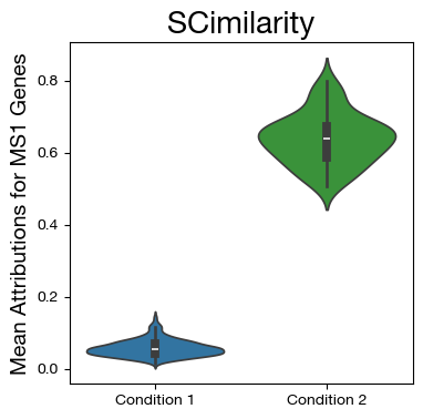
fig,ax = plt.subplots(figsize=(4,4))
sns.violinplot(data=mdf, x="disease", y="MS1", density_norm='width',
palette=["tab:blue", "tab:green"])
ax.set_title('SCimilarity', fontsize=20)
ax.set_ylabel('Mean Attributions for MS1 Genes', fontsize=14)
ax.set_xlabel('')
[17]:
Text(0.5, 0, '')
scFoundation#
First, calculating attributions with scFoundation requires installing two additional packages (“einops==0.8.1” and “local-attention==1.11.2”)
To use scFoundation, download the pre-trained models folder. Then download the models.ckpt file from here and put into scfoundation folder.
[18]:
from SIGnature.models.scfoundation import SCFoundationWrapper

model_path = join(base_model_fold, "scfoundation")
scf = SCFoundationWrapper(model_path=model_path, use_gpu=True)
{'mask_gene_name': False, 'gene_num': 19266, 'seq_len': 19266, 'encoder': {'hidden_dim': 768, 'depth': 12, 'heads': 12, 'dim_head': 64, 'seq_len': 19266, 'module_type': 'transformer', 'norm_first': False}, 'decoder': {'hidden_dim': 512, 'depth': 6, 'heads': 8, 'dim_head': 64, 'module_type': 'performer', 'seq_len': 19266, 'norm_first': False}, 'n_class': 104, 'pad_token_id': 103, 'mask_token_id': 102, 'bin_num': 100, 'bin_alpha': 1.0, 'rawcount': True, 'model': 'mae_autobin', 'test_valid_train_idx_dict': '/nfs_beijing/minsheng/data/os10000w-new/global_shuffle/meta.csv.train_set_idx_dict.pt', 'valid_data_path': '/nfs_beijing/minsheng/data/valid_count_10w.npz', 'num_tokens': 13, 'train_data_path': None, 'isPanA': False, 'isPlanA1': False, 'max_files_to_load': 5, 'bin_type': 'auto_bin', 'value_mask_prob': 0.3, 'zero_mask_prob': 0.03, 'replace_prob': 0.8, 'random_token_prob': 0.1, 'mask_ignore_token_ids': [0], 'decoder_add_zero': True, 'mae_encoder_max_seq_len': 15000, 'isPlanA': False, 'mask_prob': 0.3, 'model_type': 'mae_autobin', 'pos_embed': False, 'device': 'cuda'}
[19]:
tadata = scf.preprocess_adata(adata.copy())
[20]:
# replace "ig" (integrated gradients) with "dl" (deeplift) or "ixg" (input x gradients) for other methods.
# batch size set to 1 for scfoundation due to memory constraints
atts = scf.calculate_attributions(tadata.X, batch_size=1, method="ig")
100%|██████████| 550/550 [05:32<00:00, 1.65it/s]
[21]:
mdf = tadata.obs.copy()
mgenes = tadata.var.index.tolist()
gi = [mgenes.index(x) for x in ms1_genes if x in mgenes]
mdf["MS1"] = atts[:, gi].mean(axis=1)
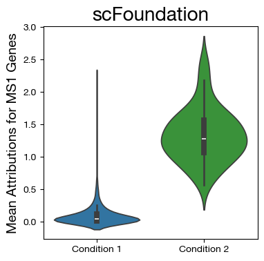
fig,ax = plt.subplots(figsize=(4,4))
sns.violinplot(data=mdf, x="disease", y="MS1", density_norm='width',
palette=["tab:blue", "tab:green"])
ax.set_title('scFoundation', fontsize=20)
ax.set_ylabel('Mean Attributions for MS1 Genes', fontsize=14)
ax.set_xlabel('')
[21]:
Text(0.5, 0, '')
SSL-scTab#
To use SSL models, download the pre-trained models folder. Individual models can then be downloaded from here
scTab RandomMask Constrastive Loss#
To use this model, download “RandomMask.ckpt” from here and put in SSL folder.
[22]:
from SIGnature.models.ssl import SSLWrapper

model_path = join(base_model_fold, "ssl")
ssl = SSLWrapper(model_path=model_path, model_filename="RandomMask.ckpt", use_gpu=True)
[23]:
tadata = ssl.preprocess_adata(adata.copy())
[24]:
# replace "ig" (integrated gradients) with "dl" (deeplift) or "ixg" (input x gradients) for other methods.
atts = ssl.calculate_attributions(
    tadata.X, batch_size=100, method="ig"
)
100%|██████████| 6/6 [00:00<00:00, 7.76it/s]
[25]:
mdf = tadata.obs.copy()
mgenes = tadata.var.index.tolist()
gi = [mgenes.index(x) for x in ms1_genes if x in mgenes]
mdf["MS1"] = atts[:, gi].mean(axis=1)
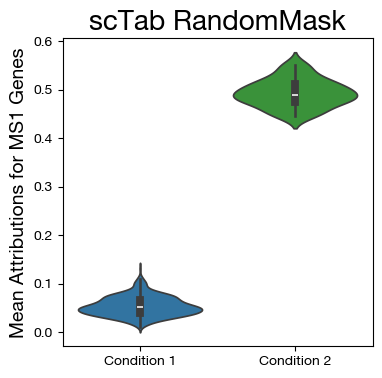
fig,ax = plt.subplots(figsize=(4,4))
sns.violinplot(data=mdf, x="disease", y="MS1", density_norm='width',
palette=["tab:blue", "tab:green"])
ax.set_title('scTab RandomMask', fontsize=20)
ax.set_ylabel('Mean Attributions for MS1 Genes', fontsize=14)
ax.set_xlabel('')
[25]:
Text(0.5, 0, '')
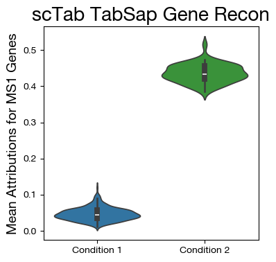
Gene Reconstruction FineTuned Model#
To use this model, download “Tabula_Sapiens_Supervised.ckpt” from here, rename it “Tabula_Sapiens_SSL_GR.ckpt”, and put it in SSL folder.
[26]:
from SIGnature.models.ssl import SSLWrapper

model_path = join(base_model_fold, "ssl")
ssl = SSLWrapper(model_path=model_path, model_filename="Tabula_Sapiens_SSL_GR.ckpt", use_gpu=True)
[27]:
tadata = ssl.preprocess_adata(adata.copy())
[28]:
# replace "ig" (integrated gradients) with "dl" (deeplift) or "ixg" (input x gradients) for other methods.
atts = ssl.calculate_attributions(
    tadata.X, batch_size=100, method="ig"
)
100%|██████████| 6/6 [00:00<00:00, 8.02it/s]
[29]:
mdf = tadata.obs.copy()
mgenes = tadata.var.index.tolist()
gi = [mgenes.index(x) for x in ms1_genes if x in mgenes]
mdf["MS1"] = atts[:, gi].mean(axis=1)

fig,ax = plt.subplots(figsize=(4,4))
sns.violinplot(data=mdf, x="disease", y="MS1", density_norm='width',
palette=["tab:blue", "tab:green"])
ax.set_title('scTab TabSap Gene Recon', fontsize=20)
ax.set_ylabel('Mean Attributions for MS1 Genes', fontsize=14)
ax.set_xlabel('')
[29]:
Text(0.5, 0, '')
Cell Type FineTuned Model#
To use this model, download “Tabula_Sapiens_Supervised.ckpt” from here, rename it “Tabula_Sapiens_SSL_CT.ckpt”, and put it in SSL folder.
[24]:
from SIGnature.models.ssl import SSLWrapper

model_path = join(base_model_fold, "ssl")
ssl = SSLWrapper(model_path=model_path, model_filename="Tabula_Sapiens_SSL_CT.ckpt",
use_gpu=True)
[25]:
tadata = ssl.preprocess_adata(adata.copy())
[26]:
# replace "ig" (integrated gradients) with "dl" (deeplift) or "ixg" (input x gradients) for other methods.
atts = ssl.calculate_attributions(
    tadata.X, batch_size=100, method="ig"
)
100%|██████████| 6/6 [00:00<00:00, 10.59it/s]
[27]:
mdf = tadata.obs.copy()
mgenes = tadata.var.index.tolist()
gi = [mgenes.index(x) for x in ms1_genes if x in mgenes]
mdf["MS1"] = atts[:, gi].mean(axis=1)

fig,ax = plt.subplots(figsize=(4,4))
sns.violinplot(data=mdf, x="disease", y="MS1", density_norm='width',
palette=["tab:blue", "tab:green"])
ax.set_title('scTab TabSap Cell Type (Emb)', fontsize=20)
ax.set_ylabel('Mean Attributions for MS1 Genes', fontsize=14)
ax.set_xlabel('')
[27]:
Text(0.5, 0, '')

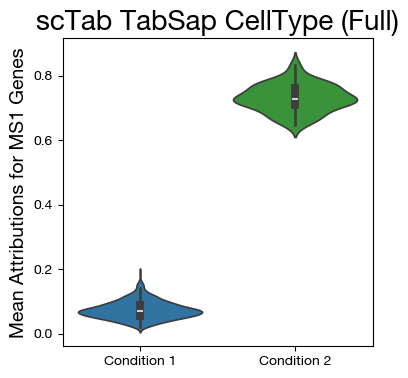
Cell Type FineTuned Model (last layer)#
To use this model, download “Tabula_Sapiens_Supervised.ckpt” from here, rename it “Tabula_Sapiens_SSL_CT.ckpt”, and put it in SSL folder.
By default, the models from the ssl_in_scg paper have 5 layers for the embedder/backbone.
If you want to calculate attributions on a different layer, you can adjust the n_layers parameter in SSL
[29]:
from SIGnature.models.ssl import SSLWrapper

model_path = join(base_model_fold, "ssl")
## consider the 6th (final classification layer)
ssl = SSLWrapper(model_path=model_path, model_filename="Tabula_Sapiens_SSL_CT.ckpt", use_gpu=True, n_layers=6)
[30]:
tadata = ssl.preprocess_adata(adata.copy())
[31]:
# replace "ig" (integrated gradients) with "dl" (deeplift) or "ixg" (input x gradients) for other methods.
# default layer is set to 12 (final layer of embedding for this structure. Can change to None to get attributions from entire final classification layer)
atts = ssl.calculate_attributions(
    tadata.X, batch_size=100, method="ig",
)
100%|██████████| 6/6 [00:00<00:00, 10.29it/s]
[32]:
mdf = tadata.obs.copy()
mgenes = tadata.var.index.tolist()
gi = [mgenes.index(x) for x in ms1_genes if x in mgenes]
mdf["MS1"] = atts[:, gi].mean(axis=1)

fig,ax = plt.subplots(figsize=(4,4))
sns.violinplot(data=mdf, x="disease", y="MS1", density_norm='width',
palette=["tab:blue", "tab:green"])
ax.set_title('scTab TabSap CellType (Full)', fontsize=20)
ax.set_ylabel('Mean Attributions for MS1 Genes', fontsize=14)
ax.set_xlabel('')
[32]:
Text(0.5, 0, '')
scVI#
To use this model, you must install scVI package to calculate attributions with scVI (“pip install scvi-tools[cuda]” for GPU or “pip install scvi-tools” for no GPU)
Then, download the scvi model of choice from here and put into scvi folder
[38]:
from SIGnature.models.scvi import SCVIWrapper

model_base = join(base_model_fold, "scvi")
model_path = join(model_base, "2023-12-15-scvi-homo-sapiens/scvi.model")
scvi = SCVIWrapper(model_path=model_path, use_gpu=True)
[39]:
tadata = scvi.preprocess_adata(
    adata.copy(), ensembl_gene_file=join(model_base, "ensembl_gene_symbols.txt")
)
INFO     File /gstore/data/omni/scdb/signature/model_files/scvi/2023-12-15-scvi-homo-sapiens/scvi.model/model.pt
         already downloaded
INFO     File /gstore/data/omni/scdb/signature/model_files/scvi/2023-12-15-scvi-homo-sapiens/scvi.model/model.pt
         already downloaded
INFO     Found 48.8375% reference vars in query data.
[40]:
# replace "ig" (integrated gradients) with "dl" (deeplift) or "ixg" (input x gradients) for other methods.
atts = scvi.calculate_attributions(
    tadata, batch_size=100, method="ig"
)
INFO     File /gstore/data/omni/scdb/signature/model_files/scvi/2023-12-15-scvi-homo-sapiens/scvi.model/model.pt
         already downloaded
100%|██████████| 6/6 [00:00<00:00, 8.92it/s]
[41]:
mdf = tadata.obs.copy()
mgenes = tadata.var.symbol.tolist()
gi = [mgenes.index(x) for x in ms1_genes if x in mgenes]
mdf["MS1"] = atts[:, gi].mean(axis=1)
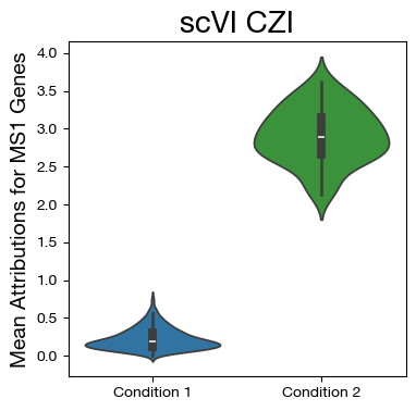
fig,ax = plt.subplots(figsize=(4,4))
sns.violinplot(data=mdf, x="disease", y="MS1", density_norm='width',
palette=["tab:blue", "tab:green"])
ax.set_title('scVI CZI', fontsize=20)
ax.set_ylabel('Mean Attributions for MS1 Genes', fontsize=14)
ax.set_xlabel('')
[41]:
Text(0.5, 0, '')