3. Specifying prior distributions

Matt Secrest and Isaac Gravestock

library(psborrow2)

In this article, you’ll learn how to specify prior distributions in psborrow2.

Specifying prior distributions

Because psborrow2 creates fully-parametrized Bayesian models, proper prior distributions on all parameters must be specified.

Prior distributions are needed for several parameters, depending on the analysis:

• beta coefficients (e.g. log hazard ratios or log odds ratios) for all coefficients, passed to add_covariates()
• ancillary parameters for outcome distributions, such as the shape parameter for the Weibull survival distribution, passed to outcome_surv_weibull_ph()
• log effect estimates (e.g. hazard ratios or odds ratios) for the primary contrast between treatments, passed to treatment_details()
• baseline outcome rates or odds, passed to outcome functions
• the hyperprior on the commensurability parameter for Bayesian dynamic borrowing (BDB), passed to borrowing_hierarchical_commensurate()

See the documentation of these functions for more information.

Types of prior distributions

The currently supported prior distributions are created with the prior_ constructors below:

• prior_bernoulli()
• prior_beta()
• prior_cauchy()
• prior_exponential()
• prior_gamma()
• prior_half_cauchy()
• prior_half_normal()
• prior_normal()
• prior_poisson()

For example, we can create an uninformative normal distribution by specifying a normal prior centered around 0 with a very large standard deviation:

uninformative_normal <- prior_normal(0, 10000)
uninformative_normal
# Normal Distribution
# Parameters:
#  Stan  R    Value
#  mu    mean     0
#  sigma sd   10000

See the documentation for the respective functions above for additional information.

Visualizing prior distributions

You may sometimes find it useful to visualize prior distributions. In these scenarios, you can call plot() on the prior object to visualize the distribution:

plot(uninformative_normal)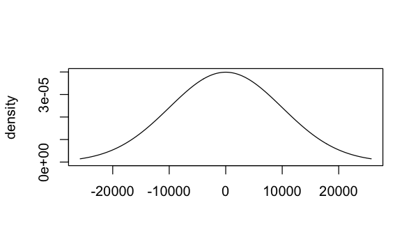

plot of chunk unnamed-chunk-3

plot() chooses the default axes for you, but you can change these to make differences more obvious. Let’s compare a conservative gamma(0.001, 0.001) hyperprior distribution on the commensurability parameter tau to an more aggressive gamma(1, 0.001) distribution with greater density at higher values of tau (which will lead to more borrowing in a BDB analysis):

conservative_tau <- prior_gamma(0.001, 0.001)
aggressive_tau <- prior_gamma(1, 0.001)
plot(aggressive_tau, xlim = c(0, 2000), col = "blue", ylim = c(0, 1e-03))
plot(conservative_tau, xlim = c(0, 2000), col = "red", add = TRUE)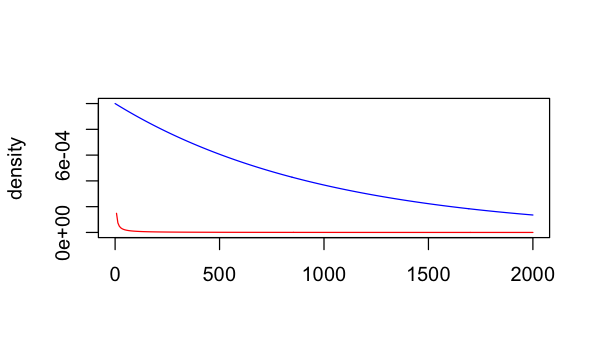

plot of chunk unnamed-chunk-4