8. Data Simulation

This vignette will show the internal functions for generating data that can be used in simulation studies.

library(psborrow2)
#> Loading required package: cmdstanr
#> CmdStan path set to: /root/.cmdstan/cmdstan-2.33.1
#> This is cmdstanr version 0.6.1
#> - CmdStanR documentation and vignettes: mc-stan.org/cmdstanr
#> - CmdStan path: /root/.cmdstan/cmdstan-2.33.1
#> - CmdStan version: 2.33.1

Generating Baseline Data

First we define how to generate baseline data for our study. In its simplest form we only need to define how many patients are in the arms: treated internal, control internal, control external.

simple_baseline <- create_baseline_object(
  n_trt_int = 100,
  n_ctrl_int = 50,
  n_ctrl_ext = 100
)

This object defines how the data will be created. To actually generate a sample, use generate() to produce a data.frame.

generate(simple_baseline)
#>   patid ext trt
#> 1     1   0   1
#> 2     2   0   1
#> 3     3   0   1
#> 4     4   0   1
#> 5     5   0   1
#> 6     6   0   1
#>  [ reached 'max' / getOption("max.print") -- omitted 244 rows ]

Often we are interested in some additional covariates. Internally the package uses multivariate normal distributions, so we need to specify the mean and (co-)variance. We have the option to specify different distribution parameters for the internal and external arms. The internal arms are assumed to be randomized and therefore come from the same distribution. If no external parameters are specified, the internal ones are used for both.

with_age <- create_baseline_object(
  n_trt_int = 100,
  n_ctrl_int = 50,
  n_ctrl_ext = 100,
  covariates = baseline_covariates(
    names = "age",
    means_int = 55,
    covariance_int = covariance_matrix(5)
  )
)
generate(with_age)
#>   patid ext trt      age
#> 1     1   0   1 51.11546
#> 2     2   0   1 55.41824
#> 3     3   0   1 54.91346
#> 4     4   0   1 55.83540
#> 5     5   0   1 54.94091
#>  [ reached 'max' / getOption("max.print") -- omitted 245 rows ]

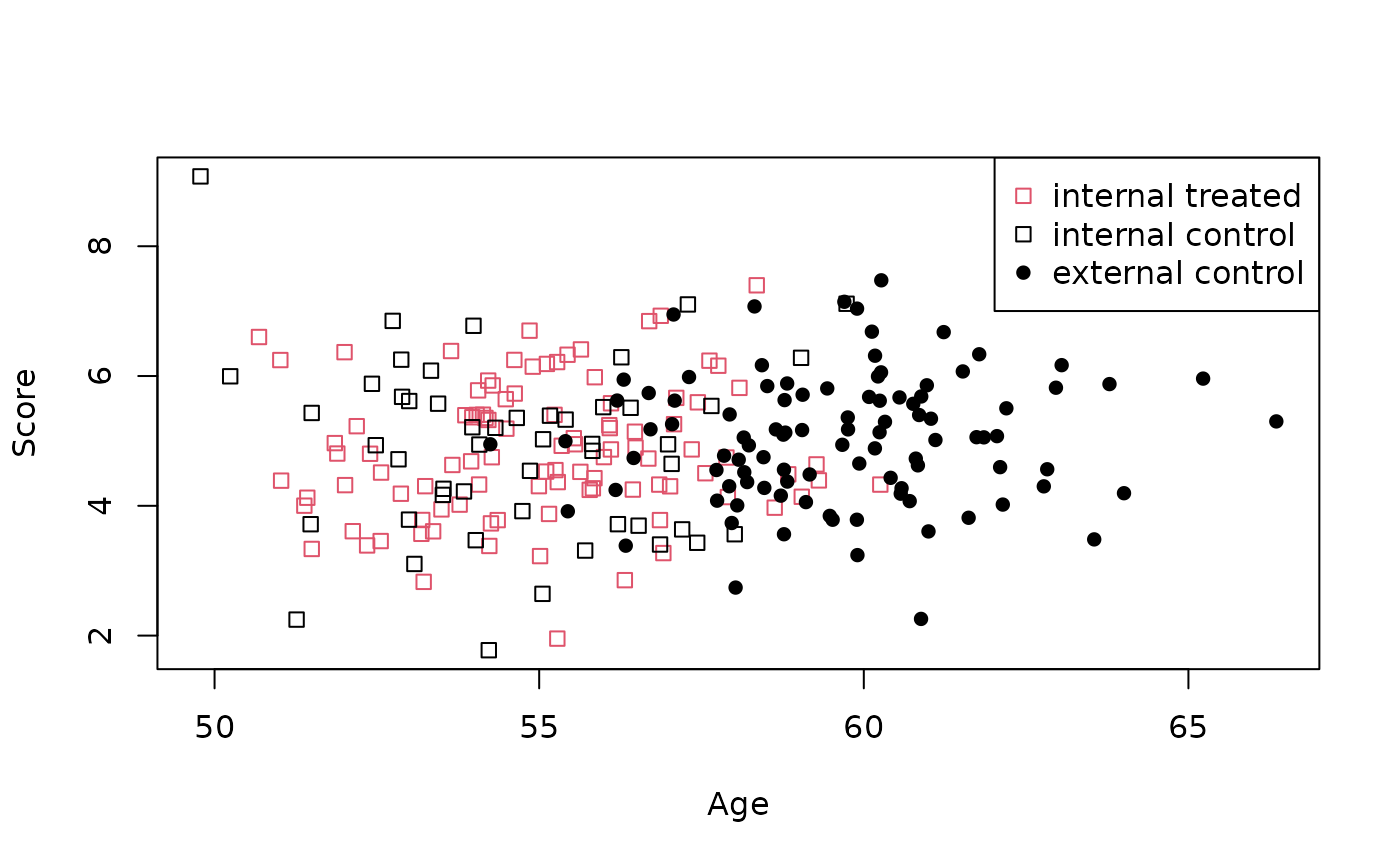
In a more complex setting, we can generate correlated baseline covariates.

with_age_score <- create_baseline_object(
  n_trt_int = 100,
  n_ctrl_int = 50,
  n_ctrl_ext = 100,
  covariates = baseline_covariates(
    names = c("age", "score"),
    means_int = c(55, 5),
    means_ext = c(60, 5),
    covariance_int = covariance_matrix(c(5, 1))
  )
)
data_age_score <- generate(with_age_score)

plot(
  x = data_age_score$age,
  y = data_age_score$score,
  col = data_age_score$trt + 1,
  pch = data_age_score$ext * 16,
  xlab = "Age",
  ylab = "Score"
)
legend(
  "topright",
  legend = c("internal treated", "internal control", "external control"),
  col = c(2, 1, 1),
  pch = c(0, 0, 16)
)

Finally, we have the option to transform non-normal covariates, such as with binary cut-offs. These can be added to existing objects and can use built-in functions or used defined.

with_age_score@transformations <- list(
  score_high = binary_cutoff("score", int_cutoff = 0.7, ext_cutoff = 0.7),
  score_rounded = function(data) round(data$score)
)
generate(with_age_score)
#>   patid ext trt      age    score score_high score_rounded
#> 1     1   0   1 53.96892 5.460058          0             5
#> 2     2   0   1 58.15331 5.078346          0             5
#>  [ reached 'max' / getOption("max.print") -- omitted 248 rows ]