5. Incorporating propensity scores analysis in psborrow2

library(psborrow2)

Propensity scores (PS) methods offer various ways to adjust analyses for differences in groups of patients. Austin (2013) discusses various approaches for using PS with survival analyses to obtain effect measures similar to randomized controlled trials. Wang et al. (2021) discuss using PS for IPTW, matching and stratification in combination with a Bayesian analysis. These methods allow for the separation of the design and analysis into two stages, which may be attractive in a regulatory setting. Another approach is the direct inclusion of the PS as a covariate in the outcome model.

Alternative PS Weights with `WeightIt`

The WeightIt package can calculate PS and other balancing weights with a number of different methods, such as generalized boosted modeling (method = "gbm"). In addition, weights can be calculated differently for different estimands. Here, we specifying estimand = "ATT", to calculate weights for estimating the average treatment effect among the treated (ATT).

library(WeightIt)

example_dataframe <- as.data.frame(example_matrix)
example_dataframe$int <- 1 - example_dataframe$ext

weightit_model <- weightit(
  int ~ cov1 + cov2 + cov3 + cov4,
  data = example_dataframe,
  method = "gbm",
  estimand = "ATT"
)
#> Warning: No `criterion` was provided. Using "smd.mean"FALSETRUE.
summary(weightit_model)
#>                  Summary of weights
#> 
#> - Weight ranges:
#> 
#>            Min                                  Max
#> treated 1.0000      ||                       1.0000
#> control 0.0826 |---------------------------| 5.8966
#> 
#> - Units with the 5 most extreme weights by group:
#>                                            
#>               5      4      3      2      1
#>  treated      1      1      1      1      1
#>             195    158    465    438    371
#>  control 2.7924 2.7924 5.8966 5.8966 5.8966
#> 
#> - Weight statistics:
#> 
#>         Coef of Var  MAD Entropy # Zeros
#> treated       0.000 0.00     0.0       0
#> control       1.582 0.82     0.6       0
#> 
#> - Effective Sample Sizes:
#> 
#>            Control Treated
#> Unweighted  350.       150
#> Weighted    100.09     150

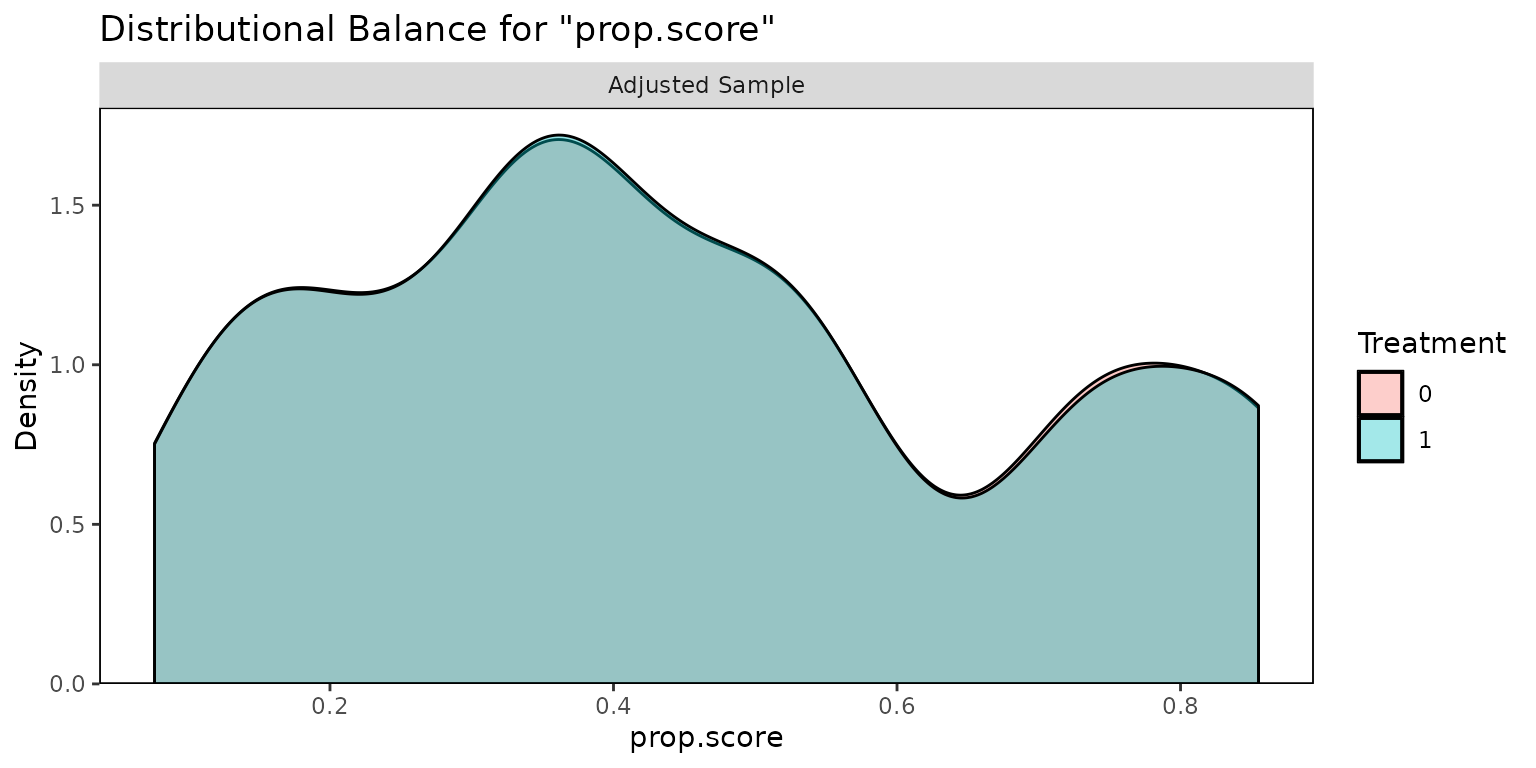
Another useful package is cobalt, which provides tools for assessing balance between groups after weighting or matching. It is compatible with many matching and weighting packages. See the vignette for more details. We can use the cobalt package to assess balance with bal.plot().

library(cobalt)
#>  cobalt (Version 4.5.1, Build Date: 2023-04-27)
bal.plot(weightit_model)
#> No `var.name` was provided. Displaying balance for prop.score.

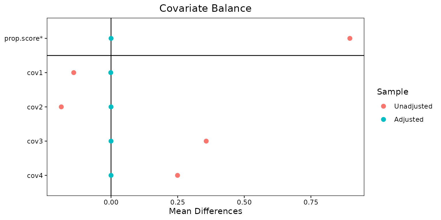
“Love plots” can also be generated that compare the populations before and after weighting:

love.plot(weightit_model, stars = "std")

The PS values can be copied into the data set and the analysis object can be constructed as before.

example_dataframe$att <- weightit_model$weights

example_matrix_att <- create_data_matrix(
  example_dataframe,
  ext_flag_col = "ext",
  outcome = c("time", "cnsr"),
  trt_flag_col = "trt",
  weight_var = "att"
)

analysis_att <- create_analysis_obj(
  data_matrix = example_matrix_att,
  outcome = exp_surv_dist("time", "cnsr", normal_prior(0, 10000), weight_var = "att"),
  borrowing = borrowing_details("Full borrowing", "ext"),
  treatment = treatment_details("trt", normal_prior(0, 10000))
)
#> Inputs look good.
#> NOTE: dropping column `ext` for full borrowing.
#> Stan program compiled successfully!
#> Ready to go! Now call `mcmc_sample()`.

result_att <- mcmc_sample(analysis_att)
#> Running MCMC with 4 sequential chains...
#> 
#> Chain 1 finished in 2.5 seconds.
#> Chain 2 finished in 2.4 seconds.
#> Chain 3 finished in 2.2 seconds.
#> Chain 4 finished in 2.5 seconds.
#> 
#> All 4 chains finished successfully.
#> Mean chain execution time: 2.4 seconds.
#> Total execution time: 9.9 seconds.

Matching with `MatchIt`

A variety of matching methods, including PS matching are implemented in the MatchIt package.

As described in the Getting Started vignette, it can be useful to check the imbalance before matching.

library(MatchIt)
#> 
#> Attaching package: 'MatchIt'
#> The following object is masked from 'package:cobalt':
#> 
#>     lalonde
# No matching; constructing a pre-match matchit object
no_match <- matchit(trt ~ cov1 + cov2 + cov3 + cov4,
  data = example_dataframe,
  method = NULL, distance = "glm"
)
summary(no_match)
#> 
#> Call:
#> matchit(formula = trt ~ cov1 + cov2 + cov3 + cov4, data = example_dataframe, 
#>     method = NULL, distance = "glm")
#> 
#> Summary of Balance for All Data:
#>          Means Treated Means Control Std. Mean Diff. Var. Ratio eCDF Mean
#> distance        0.2898        0.1776          0.7585     1.5831    0.2328
#> cov1            0.6300        0.7150         -0.1761          .    0.0850
#> cov2            0.3700        0.4625         -0.1916          .    0.0925
#> cov3            0.7600        0.4475          0.7317          .    0.3125
#> cov4            0.4600        0.2250          0.4715          .    0.2350
#>          eCDF Max
#> distance   0.3375
#> cov1       0.0850
#> cov2       0.0925
#> cov3       0.3125
#> cov4       0.2350
#> 
#> Sample Sizes:
#>           Control Treated
#> All           400     100
#> Matched       400     100
#> Unmatched       0       0
#> Discarded       0       0

Here we are matching treated to untreated to select the most comparable control group, regardless of whether they are internal or external. For simplicity let’s try a 1:1 nearest matching approach.

match_11 <- matchit(trt ~ cov1 + cov2 + cov3 + cov4,
  data = example_dataframe,
  method = "nearest", distance = "glm"
)
summary(match_11)
#> 
#> Call:
#> matchit(formula = trt ~ cov1 + cov2 + cov3 + cov4, data = example_dataframe, 
#>     method = "nearest", distance = "glm")
#> 
#> Summary of Balance for All Data:
#>          Means Treated Means Control Std. Mean Diff. Var. Ratio eCDF Mean
#> distance        0.2898        0.1776          0.7585     1.5831    0.2328
#> cov1            0.6300        0.7150         -0.1761          .    0.0850
#> cov2            0.3700        0.4625         -0.1916          .    0.0925
#> cov3            0.7600        0.4475          0.7317          .    0.3125
#> cov4            0.4600        0.2250          0.4715          .    0.2350
#>          eCDF Max
#> distance   0.3375
#> cov1       0.0850
#> cov2       0.0925
#> cov3       0.3125
#> cov4       0.2350
#> 
#> Summary of Balance for Matched Data:
#>          Means Treated Means Control Std. Mean Diff. Var. Ratio eCDF Mean
#> distance        0.2898        0.2845          0.0355     1.1082    0.0075
#> cov1            0.6300        0.6800         -0.1036          .    0.0500
#> cov2            0.3700        0.3900         -0.0414          .    0.0200
#> cov3            0.7600        0.7600          0.0000          .    0.0000
#> cov4            0.4600        0.4600          0.0000          .    0.0000
#>          eCDF Max Std. Pair Dist.
#> distance     0.07          0.0355
#> cov1         0.05          0.1036
#> cov2         0.02          0.1243
#> cov3         0.00          0.0000
#> cov4         0.00          0.0000
#> 
#> Sample Sizes:
#>           Control Treated
#> All           400     100
#> Matched       100     100
#> Unmatched     300       0
#> Discarded       0       0

plot(match_11, type = "jitter", interactive = FALSE)

Determining whether the balance after matching is appropriate is beyond the scope of this vignette. You can read more in the MatchIt Assessing Balance vignette. Again the cobalt package can be useful here.

However, if you are happy with the results of the matching procedure, you can extract the data for use in psborrow2.

example_matrix_match <- create_data_matrix(
  data = example_dataframe[match_11$weights == 1, ],
  ext_flag_col = "ext",
  outcome = c("time", "cnsr"),
  trt_flag_col = "trt"
)

analysis_match <- create_analysis_obj(
  data_matrix = example_matrix_match,
  outcome = exp_surv_dist("time", "cnsr", normal_prior(0, 10000)),
  borrowing = borrowing_details("Full borrowing", "ext"),
  treatment = treatment_details("trt", normal_prior(0, 10000))
)
#> Inputs look good.
#> NOTE: dropping column `ext` for full borrowing.
#> Stan program compiled successfully!
#> Ready to go! Now call `mcmc_sample()`.

result_match <- mcmc_sample(analysis_match)
#> Running MCMC with 4 sequential chains...
#> 
#> Chain 1 finished in 1.2 seconds.
#> Chain 2 finished in 0.9 seconds.
#> Chain 3 finished in 1.0 seconds.
#> Chain 4 finished in 1.0 seconds.
#> 
#> All 4 chains finished successfully.
#> Mean chain execution time: 1.0 seconds.
#> Total execution time: 4.4 seconds.

Combined Weighting and Dynamic Borrowing

The models also support fixed weights on the likelihood contributions from each observation. This is equivalent to fixed power prior weights. This allows for the combination of models, such as an IPTW + commensurate prior approach.

analysis_iptw_bdb <- create_analysis_obj(
  data_matrix = example_matrix_att,
  outcome = exp_surv_dist("time", "cnsr", normal_prior(0, 10000), weight_var = "att"),
  borrowing = borrowing_details("BDB", "ext", gamma_prior(0.01, 0.01)),
  treatment = treatment_details("trt", normal_prior(0, 10000))
)
#> Inputs look good.
#> Stan program compiled successfully!
#> Ready to go! Now call `mcmc_sample()`.

result_iptw_bdb <- mcmc_sample(analysis_iptw_bdb)
#> Running MCMC with 4 sequential chains...
#> 
#> Chain 1 finished in 4.2 seconds.
#> Chain 2 finished in 4.6 seconds.
#> Chain 3 finished in 4.3 seconds.
#> Chain 4 finished in 4.7 seconds.
#> 
#> All 4 chains finished successfully.
#> Mean chain execution time: 4.5 seconds.
#> Total execution time: 18.2 seconds.

Fixed Weights

We can also use weights to specify a fixed power prior model. Here we set the power parameter \(\alpha = 0.1\) for the external controls.

example_matrix_pp01 <- cbind(example_matrix, pp_alpha = ifelse(example_matrix[, "ext"] == 1, 0.1, 1))

analysis_pp01 <- create_analysis_obj(
  data_matrix = example_matrix_pp01,
  outcome = exp_surv_dist("time", "cnsr", normal_prior(0, 10000), weight_var = "pp_alpha"),
  borrowing = borrowing_details("Full borrowing", "ext"),
  treatment = treatment_details("trt", normal_prior(0, 10000))
)
#> Inputs look good.
#> NOTE: dropping column `ext` for full borrowing.
#> Stan program compiled successfully!
#> Ready to go! Now call `mcmc_sample()`.

result_pp01 <- mcmc_sample(analysis_pp01)
#> Running MCMC with 4 sequential chains...
#> 
#> Chain 1 finished in 2.8 seconds.
#> Chain 2 finished in 2.5 seconds.
#> Chain 3 finished in 2.7 seconds.
#> Chain 4 finished in 2.6 seconds.
#> 
#> All 4 chains finished successfully.
#> Mean chain execution time: 2.6 seconds.
#> Total execution time: 10.9 seconds.

Reference Models

For comparison, we also fit a full borrowing, a no borrowing, and a BDB model without weights.

result_full <- mcmc_sample(
  create_analysis_obj(
    data_matrix = example_matrix,
    outcome = exp_surv_dist("time", "cnsr", normal_prior(0, 10000)),
    borrowing = borrowing_details("Full borrowing", "ext"),
    treatment = treatment_details("trt", normal_prior(0, 10000))
  )
)
#> Inputs look good.
#> NOTE: dropping column `ext` for full borrowing.
#> Stan program compiled successfully!
#> Ready to go! Now call `mcmc_sample()`.
#> Running MCMC with 4 sequential chains...
#> 
#> Chain 1 finished in 2.0 seconds.
#> Chain 2 finished in 2.1 seconds.
#> Chain 3 finished in 2.1 seconds.
#> Chain 4 finished in 2.0 seconds.
#> 
#> All 4 chains finished successfully.
#> Mean chain execution time: 2.0 seconds.
#> Total execution time: 8.4 seconds.

result_none <- mcmc_sample(
  create_analysis_obj(
    data_matrix = example_matrix,
    outcome = exp_surv_dist("time", "cnsr", normal_prior(0, 10000)),
    borrowing = borrowing_details("No borrowing", "ext"),
    treatment = treatment_details("trt", normal_prior(0, 10000))
  )
)
#> Inputs look good.
#> NOTE: excluding `ext` == `1`/`TRUE` for no borrowing.
#> Stan program compiled successfully!
#> Ready to go! Now call `mcmc_sample()`.
#> Running MCMC with 4 sequential chains...
#> 
#> Chain 1 finished in 1.0 seconds.
#> Chain 2 finished in 0.9 seconds.
#> Chain 3 finished in 1.0 seconds.
#> Chain 4 finished in 1.0 seconds.
#> 
#> All 4 chains finished successfully.
#> Mean chain execution time: 1.0 seconds.
#> Total execution time: 4.1 seconds.

result_bdb <- mcmc_sample(
  create_analysis_obj(
    data_matrix = example_matrix_att,
    outcome = exp_surv_dist("time", "cnsr", normal_prior(0, 10000)),
    borrowing = borrowing_details("BDB", "ext", gamma_prior(0.01, 0.01)),
    treatment = treatment_details("trt", normal_prior(0, 10000))
  )
)
#> Inputs look good.
#> Stan program compiled successfully!
#> Ready to go! Now call `mcmc_sample()`.
#> Running MCMC with 4 sequential chains...
#> 
#> Chain 1 finished in 4.5 seconds.
#> Chain 2 finished in 4.3 seconds.
#> Chain 3 finished in 4.1 seconds.
#> Chain 4 finished in 5.2 seconds.
#> 
#> All 4 chains finished successfully.
#> Mean chain execution time: 4.5 seconds.
#> Total execution time: 18.4 seconds.

Comparison of Results

models <- list(
  "No borrowing" = result_none,
  "Full borrowing" = result_full,
  "Power Prior 01" = result_pp01,
  "ATT Weights" = result_att,
  "IPTW + BDB" = result_iptw_bdb,
  "Matching 1:1" = result_match,
  "BDB" = result_bdb
)

We can use summary() to extract the variable of interest and specify summary statistics.

results_table <- do.call(rbind, lapply(
  models,
  function(i) i$summary("HR_trt", c("mean", "median", "sd", "quantile2"))
))
knitr::kable(cbind(models = names(models), results_table), digits = 3)

models	variable	mean	median	sd	q5	q95
No borrowing	HR_trt	0.897	0.877	0.180	0.638	1.218
Full borrowing	HR_trt	0.388	0.385	0.049	0.313	0.473
Power Prior 01	HR_trt	0.634	0.625	0.105	0.477	0.820
ATT Weights	HR_trt	0.895	0.888	0.127	0.698	1.115
IPTW + BDB	HR_trt	0.893	0.879	0.162	0.653	1.180
Matching 1:1	HR_trt	0.794	0.784	0.129	0.600	1.023
BDB	HR_trt	0.871	0.853	0.174	0.619	1.185

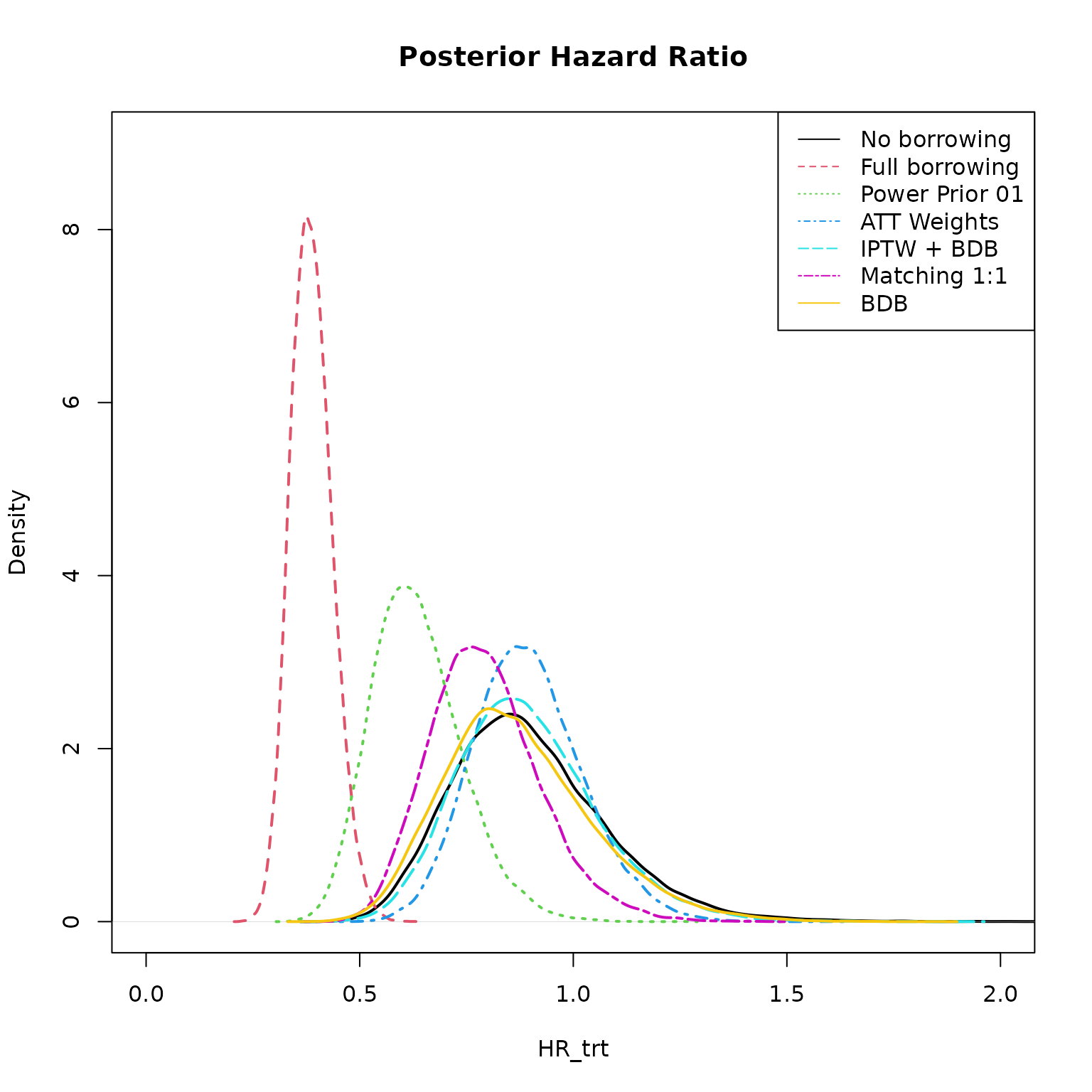
We can extract a draws object from each model and plot the posterior distribution of the treatment hazard ratio.

plot(density(models[[1]]$draws("HR_trt")),
  col = 1, xlim = c(0, 2), ylim = c(0, 9), lwd = 2,
  xlab = "HR_trt",
  main = "Posterior Hazard Ratio"
)
for (i in 2:7) {
  lines(density(models[[i]]$draws("HR_trt")), col = i, lty = i, lwd = 2)
}
legend("topright", col = seq_along(models), lty = seq_along(models), legend = names(models))

Here we see no borrowing and full borrowing at the extremes and the other methods in between.

References

Austin, Peter C. 2013. “The Use of Propensity Score Methods with Survival or Time-to-Event Outcomes: Reporting Measures of Effect Similar to Those Used in Randomized Experiments.” Statistics in Medicine 33 (7): 1242–58. https://doi.org/10.1002/sim.5984.

Wang, Xi, Leah Suttner, Thomas Jemielita, and Xiaoyun Li. 2021. “Propensity Score-Integrated Bayesian Prior Approaches for Augmented Control Designs: A Simulation Study.” Journal of Biopharmaceutical Statistics 32 (1): 170–90. https://doi.org/10.1080/10543406.2021.2011743.

Isaac Gravestock and Matt Secrest

Alternative PS Weights with WeightIt