Example application of quipcell to human lung cell atlas

In this vignette, we demonstrate the application of quipcell to bulk deconvolution, replicating some analyses from the manuscript.

For our dataset, we use the Human Lung Cell Atlas, which consists of several studies. We hold out one of the studies as a test set, which we use to generate (pseudo)bulk samples with known ground truth.

To make this analysis runnable on a laptop, the data has been preprocessed into a smaller form (just the raw counts of the highly variable genes). See the vignette readme for instructions on how to download or generate the preprocessed data before running this notebook.

from collections import Counter

import logging
logging.basicConfig(level=logging.INFO)

import numpy as np
import pandas as pd

import plotnine as gg
import mizani
import mizani.transforms as scales

import anndata as ad
import scanpy as sc

import scipy.sparse

from sklearn.discriminant_analysis import LinearDiscriminantAnalysis
from sklearn.preprocessing import OneHotEncoder

import quipcell as qpc

WARNING:matplotlib.font_manager:Matplotlib is building the font cache; this may take a moment.
INFO:matplotlib.font_manager:Failed to extract font properties from /System/Library/Fonts/Supplemental/NISC18030.ttf: In FT2Font: Could not set the fontsize (invalid pixel size; error code 0x17)
INFO:matplotlib.font_manager:Failed to extract font properties from /System/Library/Fonts/LastResort.otf: tuple indices must be integers or slices, not str
INFO:matplotlib.font_manager:Failed to extract font properties from /System/Library/Fonts/Apple Color Emoji.ttc: In FT2Font: Could not set the fontsize (invalid pixel size; error code 0x17)
INFO:matplotlib.font_manager:generated new fontManager

Load single cell data

First, we load the (preprocessed) Human Lung Cell Atlas data.

adata = ad.read_h5ad("data/hlca_hvgs.h5ad")

Next, we subset to 1/8th of the dataset to improve speed. We also exclude one of the studies as a validation test set to benchmark bulk deconvolution.

validation_study = 'Krasnow_2020'

rng = np.random.default_rng(12345)
n = adata.obs.shape[0]

keep = adata.obs['study'] != validation_study
keep = keep & (rng.random(size=n) < .125)

adata_ref = adata[keep,:]
print(f"{adata_ref.shape[0]} cells in reference set")

65531 cells in reference set

Normalize and transform single cell data

Next, normalize the raw counts. The preprocessing script saved the total UMIs per cell before filtering to highly variable genes, so we divide it out, and normalize to counts per 1000 UMIs.

# Normalize
normalize_sum = 1000
adata_ref.X = scipy.sparse.diags(normalize_sum / adata_ref.obs['n_umi'].values) @ adata_ref.X

Next, we run PCA, and then perform Linear Discriminant Analysis on the PCs and celltype labels. This will be the embedding space we use for quipcell.

sc.pp.pca(adata_ref, n_comps=100)

# since the PCA is zero-centered, we need to save the gene-wise means
# to apply PCA rotation to pseudobulks
gene_means = adata_ref.X.mean(axis=0)
gene_means = np.squeeze(np.asarray(gene_means))
adata_ref.var['x_mean'] = gene_means

lda = LinearDiscriminantAnalysis(n_components=15)

X = adata_ref.obsm['X_pca']
y = adata_ref.obs['ann_finest_level']

lda.fit(X, y)

adata_ref.obsm['X_lda'] = lda.transform(adata_ref.obsm['X_pca'])

/Users/kammj2/miniforge3/envs/quipcell/lib/python3.12/site-packages/scanpy/preprocessing/_pca.py:314: ImplicitModificationWarning: Setting element `.obsm['X_pca']` of view, initializing view as actual.

Load and transform (pseudo)bulk data

Next, we read in the pseudobulk counts (generated in preprocessing.py), and subset to the samples in the validation/test set.

We then normalize the counts, and subset to the same genes as the reference single cell set.

Then, we apply a linear transformation to map the bulk samples to the embedding space.

adata_pseudobulk = ad.read_h5ad("data/pseudobulks.h5ad")

# Subset to validation set
keep = adata_pseudobulk.obs['study'] == validation_study
adata_pseudobulk = adata_pseudobulk[keep,:]

# Normalize on the same scale as the single cell reference set
adata_pseudobulk.raw = adata_pseudobulk
sc.pp.normalize_total(adata_pseudobulk, target_sum=normalize_sum)

# Subset to same genes as the single cell reference set
adata_pseudobulk = adata_pseudobulk[:, adata.var.index]

# Apply PCA rotation to pseudobulks
X = adata_pseudobulk.X - adata_ref.var['x_mean'].values
X = np.asarray(X @ adata_ref.varm['PCs'])
adata_pseudobulk.obsm['X_pca'] = X
# Apply LDA rotation to pseudobulks
adata_pseudobulk.obsm['X_lda'] = lda.transform(X)

/var/folders/rw/hpynwn2500q6m7_3rdsw2zcc0000gp/T/ipykernel_23386/4126115140.py:17: ImplicitModificationWarning: Setting element `.obsm['X_pca']` of view, initializing view as actual.

Estimate weights for read-level abundances

Now that the single cell reference set and the bulk samples are in the same embedding space, we can estimate the weights with quipcell.

w_umi = qpc.estimate_weights_multisample(adata_ref.obsm['X_lda'],
                                         adata_pseudobulk.obsm['X_lda'])

INFO:quipcell._solvers:Solving for sample i=0
INFO:quipcell._solvers:objective=2.208068696366285, optimal
INFO:quipcell._solvers:Solving for sample i=1
INFO:quipcell._solvers:objective=1.3962415069956384, optimal
INFO:quipcell._solvers:Solving for sample i=2
INFO:quipcell._solvers:objective=2.1952911740312, optimal
INFO:quipcell._solvers:Solving for sample i=3
INFO:quipcell._solvers:objective=1.071730756157023, optimal
INFO:quipcell._solvers:Solving for sample i=4
INFO:quipcell._solvers:objective=0.4401995928507547, optimal

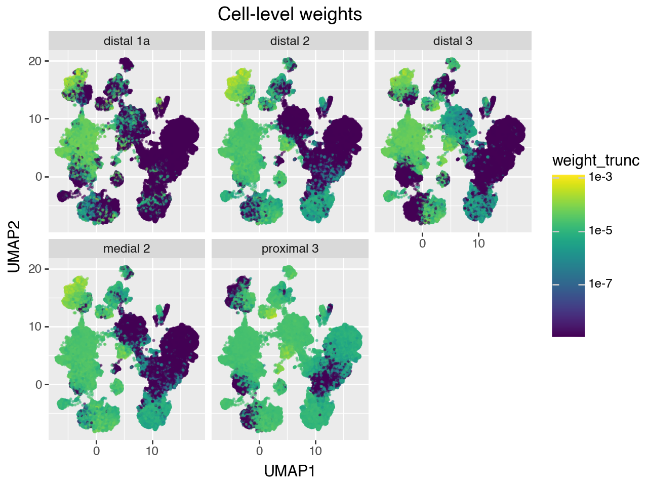
Convert read-level abundance to cell-level abundance

Note that the gene counts of bulk samples don’t normalize for the fact that different cell types have different number of reads. Therefore, the weights represent a probability distribution of a random read drawn from the bulk sample, rather than a probability distribution over a random cell from the bulk sample.

We can convert the read-level weights to cell-level weights by estimating size factors for each of the reference cells, and normalizing the weights by those.

If the reference set doesn’t have too much technical variation, then we can just use the number of UMIs per cell as the normalizing factor. However, the HLCA is a highly heterogeneous dataset, consisting of many samples from different studies, sequenced to different depths, and containing different celltypes. Therefore, we need to control for sample when estimating the size factors. quipcell provides a method to estimate size factors while controlling for sample by using Poisson regression.

# Estimate size factors using Poisson regression
size_factors = qpc.estimate_size_factors(
    adata_ref.obsm['X_lda'],
    adata_ref.obs['n_umi'].values,
    adata_ref.obs['sample'].values,
    #verbose=True
)

# Convert read-level weights to cell-level weights
w_cell = qpc.renormalize_weights(w_umi, size_factors)

/Users/kammj2/miniforge3/envs/quipcell/lib/python3.12/site-packages/sklearn/linear_model/_linear_loss.py:294: RuntimeWarning: invalid value encountered in matmul
/Users/kammj2/miniforge3/envs/quipcell/lib/python3.12/site-packages/sklearn/linear_model/_linear_loss.py:294: RuntimeWarning: invalid value encountered in matmul

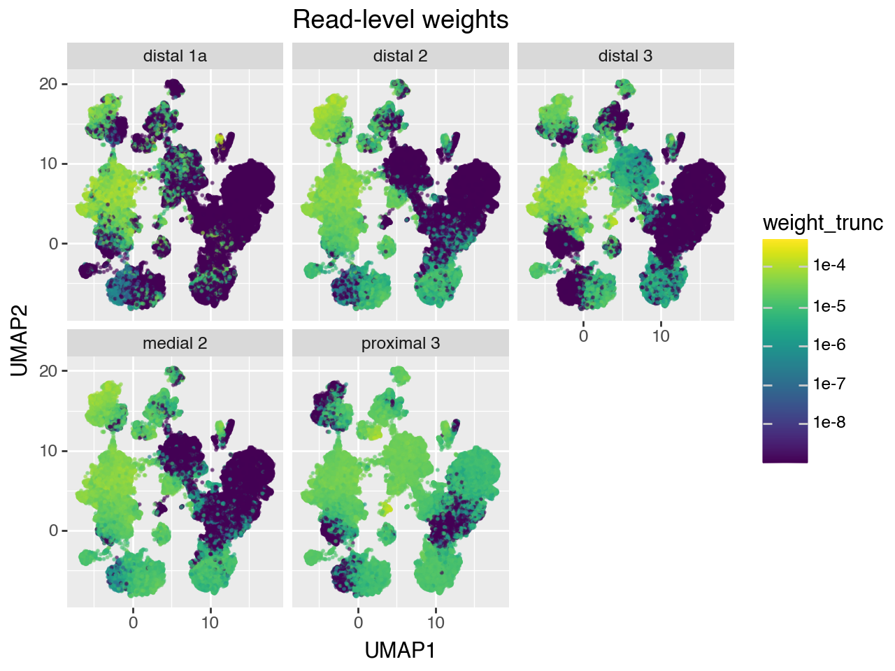
Plot inferred weights

Below, we plot the read-level and cell-level weights on the reference UMAP for each of the 5 validation bulk samples.

# Dataframe for plotting UMI-level weights on UMAP
df = pd.DataFrame(
    np.hstack([adata_ref.obsm['X_umap'], w_umi]),
    columns = ['UMAP1', 'UMAP2'] + list(adata_pseudobulk.obs.index)
).melt( # pivot to long format
    id_vars=['UMAP1', 'UMAP2'],
    var_name='sample',
    value_name='weight'
)

# set very small weights to 0 for prettier plotting
weight_trunc = df['weight'].values.copy()
weight_trunc[weight_trunc < 1e-9] = 0
df['weight_trunc'] = weight_trunc

(gg.ggplot(df, gg.aes(x="UMAP1", y="UMAP2", color="weight_trunc")) +
    gg.geom_point(size=.25, alpha=.5) +
    gg.facet_wrap("~sample") +
    gg.scale_color_cmap(trans=scales.log_trans(base=10)) +
    gg.ggtitle("Read-level weights"))

/Users/kammj2/miniforge3/envs/quipcell/lib/python3.12/site-packages/pandas/core/arraylike.py:399: RuntimeWarning: divide by zero encountered in log10
INFO:matplotlib.font_manager:Fontsize 0.00 < 1.0 pt not allowed by FreeType. Setting fontsize = 1 pt

 # Dataframe for plotting cell-level weights on UMAP
df = pd.DataFrame(
    np.hstack([adata_ref.obsm['X_umap'], w_cell]),
    columns = ['UMAP1', 'UMAP2'] + list(adata_pseudobulk.obs.index)
).melt( # pivot to long format
    id_vars=['UMAP1', 'UMAP2'],
    var_name='sample',
    value_name='weight'
)

# set very small weights to 0 for prettier plotting
weight_trunc = df['weight'].values.copy()
weight_trunc[weight_trunc < 1e-9] = 0
df['weight_trunc'] = weight_trunc

(gg.ggplot(df, gg.aes(x="UMAP1", y="UMAP2", color="weight_trunc")) +
    gg.geom_point(size=.25, alpha=.5) +
    gg.facet_wrap("~sample") +
    gg.scale_color_cmap(trans=scales.log_trans(base=10)) +
    gg.ggtitle("Cell-level weights"))

/Users/kammj2/miniforge3/envs/quipcell/lib/python3.12/site-packages/pandas/core/arraylike.py:399: RuntimeWarning: divide by zero encountered in log10
INFO:matplotlib.font_manager:Fontsize 0.00 < 1.0 pt not allowed by FreeType. Setting fontsize = 1 pt

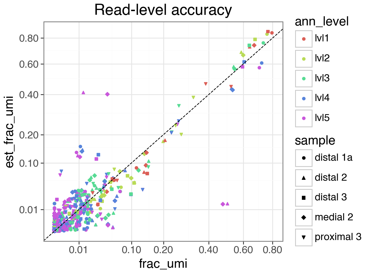
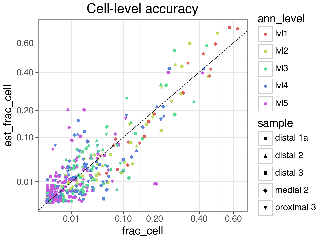
Plot true vs estimated abundances

Next, we compare the estimated weights to the true celltype proportions. In the preprocessing script, we precomputed the fraction of reads and cells coming from each celltype, at different levels of celltype annotation. We read in these precomputed abundances below.

df_abundance = pd.read_csv('data/abundances.csv')
# filter to samples in the validation set
df_abundance = df_abundance[df_abundance['sample'].isin(adata_pseudobulk.obs.index)]
# convert sample name to string to prevent missing categorical levels
df_abundance['sample'] = df_abundance['sample'].astype(str)
df_abundance

	sample	ann_level	celltype	n_umi	frac_umi	n_cell	frac_cell
644	distal 1a	lvl1	Endothelial	4461681	0.060048	1495	0.198724
645	distal 1a	lvl1	Epithelial	8394719	0.112981	853	0.113386
646	distal 1a	lvl1	Immune	59114660	0.795600	4719	0.627276
647	distal 1a	lvl1	Stroma	2330951	0.031371	456	0.060614
648	distal 2	lvl1	Endothelial	30078564	0.205619	8449	0.455693
...	...	...	...	...	...	...	...
25559	proximal 3	lvl5	Subpleural fibroblasts	0	0.000000	0	0.000000
25560	proximal 3	lvl5	Suprabasal	10395727	0.130773	482	0.062041
25561	proximal 3	lvl5	T cells proliferating	34048	0.000428	1	0.000129
25562	proximal 3	lvl5	Tuft	0	0.000000	0	0.000000
25563	proximal 3	lvl5	pre-TB secretory	1892948	0.023812	144	0.018535

770 rows × 7 columns

Next, we compute estimated celltype abundances, by summing over the weights fit by quipcell. We add the estimated number of reads and cells coming from each celltype to the dataframe of abundances.

est_frac_umi = []
est_frac_cells = []

# TODO use a more descriptive variable name than i
for i in range(1, 6):
    enc = OneHotEncoder()
    mat_onehot = enc.fit_transform(
        adata_ref.obs[f'celltype_lvl{i}'].values.reshape(-1,1)
    )

    # Function to sum weights by celltype, then pivot to long dataframe
    def aggregate_and_reshape(w):
        return pd.DataFrame(
            w.T @ mat_onehot,
            columns = enc.categories_[0],
            index = adata_pseudobulk.obs.index
        ).reset_index(names='sample').melt(
            id_vars=['sample'], var_name='celltype', value_name='weight'
        ).assign(ann_level=f'lvl{i}')

    est_frac_umi.append(aggregate_and_reshape(w_umi))
    est_frac_cells.append(aggregate_and_reshape(w_cell))


# Function to combine the summed weights across annotation levels,
# returning a vector to be added to df_abundance
def concat_aggregated_weights(agg_weight_list):
    idx_keys = ['ann_level', 'sample', 'celltype']
    return (pd.concat(agg_weight_list)
            .set_index(idx_keys)
            .loc[zip(*[df_abundance[k] for k in idx_keys])]
            .values)

df_abundance['est_frac_umi'] = concat_aggregated_weights(est_frac_umi)
df_abundance['est_frac_cell'] = concat_aggregated_weights(est_frac_cells)

df_abundance

	sample	ann_level	celltype	n_umi	frac_umi	n_cell	frac_cell	est_frac_umi	est_frac_cell
644	distal 1a	lvl1	Endothelial	4461681	0.060048	1495	0.198724	0.055587	0.184202
645	distal 1a	lvl1	Epithelial	8394719	0.112981	853	0.113386	0.085862	0.085786
646	distal 1a	lvl1	Immune	59114660	0.795600	4719	0.627276	0.843633	0.710039
647	distal 1a	lvl1	Stroma	2330951	0.031371	456	0.060614	0.014919	0.019973
648	distal 2	lvl1	Endothelial	30078564	0.205619	8449	0.455693	0.177143	0.379683
...	...	...	...	...	...	...	...	...	...
25559	proximal 3	lvl5	Subpleural fibroblasts	0	0.000000	0	0.000000	0.000464	0.000488
25560	proximal 3	lvl5	Suprabasal	10395727	0.130773	482	0.062041	0.036868	0.029626
25561	proximal 3	lvl5	T cells proliferating	34048	0.000428	1	0.000129	0.000636	0.001184
25562	proximal 3	lvl5	Tuft	0	0.000000	0	0.000000	0.000277	0.000255
25563	proximal 3	lvl5	pre-TB secretory	1892948	0.023812	144	0.018535	0.007603	0.006743

770 rows × 9 columns

Finally, we plot the estimated vs actual abundances, at both the read and cell level.

At the finest resolution (annotation level 5), there is some inaccuracy because a common celltype in the validation set (CCL3+ Alveolar macrophages) is very rare in the reference samples, and cannot be distinguished from other Alveolar macrophages in the embedding space. See the manuscript for more details.

 (gg.ggplot(df_abundance.sample(frac=1, random_state=42),
           gg.aes(x="frac_umi", y="est_frac_umi", color="ann_level", shape="sample")) +
    gg.geom_point() +
    gg.geom_abline(linetype='dashed') +
    gg.scale_x_sqrt(breaks=[.01,.1,.2,.4,.6,.8]) +
    gg.scale_y_sqrt(breaks=[.01,.1,.2,.4,.6,.8]) +
    gg.theme_bw(base_size=16) +
    gg.ggtitle("Read-level accuracy"))

INFO:matplotlib.font_manager:Fontsize 0.00 < 1.0 pt not allowed by FreeType. Setting fontsize = 1 pt

 (gg.ggplot(df_abundance.sample(frac=1, random_state=42),
           gg.aes(x="frac_cell", y="est_frac_cell", color="ann_level", shape="sample")) +
    gg.geom_point() +
    gg.geom_abline(linetype='dashed') +
    gg.scale_x_sqrt(breaks=[.01,.1,.2,.4,.6,.8]) +
    gg.scale_y_sqrt(breaks=[.01,.1,.2,.4,.6,.8]) +
    gg.theme_bw(base_size=16) +
    gg.ggtitle("Cell-level accuracy"))

INFO:matplotlib.font_manager:Fontsize 0.00 < 1.0 pt not allowed by FreeType. Setting fontsize = 1 pt