Purpose
The goal of this demo is to conduct a Bayesian Dynamic Borrowing (BDB) analysis using the hierarchical commensurate prior on a dataset.
# Load packages ----
library(psborrow2)

# Survival analysis
library(survival)
library(ggsurvfit)
library(flexsurv)

# Additional tools for draws objects
library(bayesplot)
library(posterior)

# Comparing populations
library(table1)
Explore example data
{psborrow2} contains an example matrix
head(example_matrix)## id ext trt cov4 cov3 cov2 cov1 time status cnsr resp
## [1,] 1 0 0 1 1 1 0 2.4226411 1 0 1
## [2,] 2 0 0 1 1 0 1 50.0000000 0 1 1
## [3,] 3 0 0 0 0 0 1 0.9674372 1 0 1
## [4,] 4 0 0 1 1 0 1 14.5774738 1 0 1
## [5,] 5 0 0 1 1 0 0 50.0000000 0 1 0
## [6,] 6 0 0 1 1 0 1 50.0000000 0 1 0?example_matrix # for more detailsLoad as data.frame for some functions
example_dataframe <- as.data.frame(example_matrix)Look at distribution of arms
table(ext = example_matrix[, "ext"], trt = example_matrix[, "trt"])## trt
## ext 0 1
## 0 50 100
## 1 350 0Naive internal comparisons
Kaplan-Meier curves
km_fit <- survfit(Surv(time = time, event = 1 - cnsr) ~ trt + ext,
  data = example_dataframe
)

ggsurvfit(km_fit)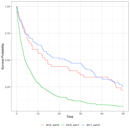
The internal and external control arms look quite different…
Cox model
cox_fit <- coxph(Surv(time = time, event = 1 - cnsr) ~ trt,
  data = example_dataframe,
  subset = ext == 0
)

cox_fit
## Call:
## coxph(formula = Surv(time = time, event = 1 - cnsr) ~ trt, data = example_dataframe,
## subset = ext == 0)
##
## coef exp(coef) se(coef) z p
## trt -0.1097 0.8961 0.1976 -0.555 0.579
##
## Likelihood ratio test=0.3 on 1 df, p=0.5809
## n= 150, number of events= 114## 2.5 % 97.5 %
## trt 0.6083595 1.319842Hybrid control analysis
Let’s start by demonstrating the utility of BDB by trying to borrow data from the external control arm which we know experiences worse survival.
The end goal is to create an Analysis object with:
?create_analysis_objA note on prior distributions
psborrow2 allows the user to specify priors with the following functions:
?prior_bernoulli
?prior_beta
?prior_cauchy
?prior_exponential
?prior_gamma
?prior_normal
?prior_poisson
?prior_uniform
Prior distributions can be plotted with the plot() method
plot(prior_normal(0, 1), xlim = c(-100, 100), ylim = c(0, 1))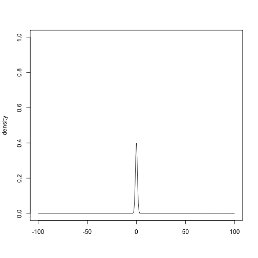
plot(prior_normal(0, 10), xlim = c(-100, 100), ylim = c(0, 1))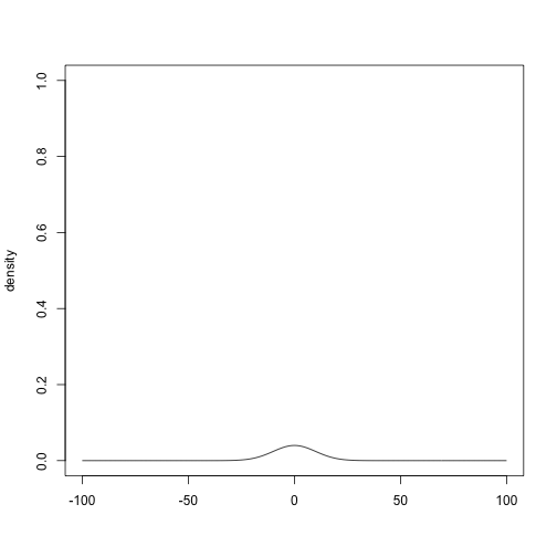
plot(prior_normal(0, 10000), xlim = c(-100, 100), ylim = c(0, 1))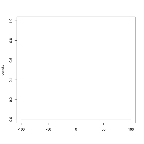
Outcome objects
psborrow2 currently supports 4 outcomes:
?outcome_surv_weibull_ph # Weibull survival w/ proportional hazards
?outcome_surv_exponential # Exponential survival
?outcome_bin_logistic # Logistic binary outcome
?outocme_cont_normal # Normal continuous outcome
Create an exponential survival distribution Outcome object
exp_outcome <- outcome_surv_exponential(
  time_var = "time",
  cens_var = "cnsr",
  baseline_prior = prior_normal(0, 10000)
)
Borrowing object
Borrowing objects are created with:
?borrowing_hierarchical_commensurate # Hierarchical commensurate borrowing
?borrowing_none # No borrowing
?borrowing_full # Full borrowing
bdb_borrowing <- borrowing_hierarchical_commensurate(
  ext_flag_col = "ext",
  tau_prior = prior_gamma(0.001, 0.001)
)
Treatment objects
Treatment objects are created with:
?treatment_details
trt_details <- treatment_details(
  trt_flag_col = "trt",
  trt_prior = prior_normal(0, 10000)
)
Analysis objects
Combine everything and create object of class Analysis:
analysis_object <- create_analysis_obj(
  data_matrix = example_matrix,
  outcome = exp_outcome,
  borrowing = bdb_borrowing,
  treatment = trt_details
)
## Inputs look good.## Stan program compiled successfully!## Ready to go! Now call `mcmc_sample()`.
analysis_object## Analysis Object
##
## Outcome model: OutcomeSurvExponential
## Outcome variables: time cnsr
##
## Borrowing method: Bayesian dynamic borrowing with the hierarchical commensurate prior
## External flag: ext
##
## Treatment variable: trt
##
## Data: Matrix with 500 observations
## - 50 internal controls
## - 350 external controls
## - 100 internal experimental
##
## Stan model compiled and ready to sample.
## Call mcmc_sample() next.MCMC sampling
Conduct MCMC sampling with:
?mcmc_sampleresults <- mcmc_sample(
x = analysis_object,
iter_warmup = 1000,
iter_sampling = 5000,
chains = 1
)
class(results)## [1] "CmdStanMCMC" "CmdStanFit" "R6"
results## variable mean median sd mad q5 q95 rhat ess_bulk ess_tail
## lp__ -1617.98 -1617.62 1.52 1.30 -1620.95 -1616.18 1.00 1933 1780
## beta_trt -0.15 -0.16 0.20 0.20 -0.48 0.18 1.00 2167 2493
## alpha[1] -3.36 -3.36 0.16 0.16 -3.62 -3.10 1.00 2129 2970
## alpha[2] -2.40 -2.40 0.05 0.05 -2.49 -2.31 1.00 4276 3255
## tau 1.12 0.46 1.79 0.64 0.00 4.43 1.00 1650 1382
## HR_trt 0.88 0.86 0.18 0.17 0.62 1.19 1.00 2167 2493Interpret results
Dictionary to interpret parameters:
variable_dictionary(analysis_object)## Stan_variable Description
## 1 tau commensurability parameter
## 2 alpha[1] baseline log hazard rate, internal
## 3 alpha[2] baseline log hazard rate, external
## 4 beta_trt treatment log HR
## 5 HR_trt treatment HRCreate a draws object
draws <- results$draws()Rename draws object parameters
draws <- rename_draws_covariates(draws, analysis_object)Get 95% credible intervals with posterior package
posterior::summarize_draws(draws, ~ quantile(.x, probs = c(0.025, 0.50, 0.975)))## # A tibble: 6 × 4
## variable `2.5%` `50%` `97.5%`
## <chr> <dbl> <dbl> <dbl>
## 1 lp__ -1622. -1618. -1616.
## 2 treatment log HR -0.545 -0.156 0.234
## 3 baseline log hazard rate, internal -3.68 -3.36 -3.05
## 4 baseline log hazard rate, external -2.51 -2.40 -2.29
## 5 commensurability parameter 0.000452 0.456 6.14
## 6 treatment HR 0.580 0.856 1.26Look at histogram of draws with bayesplot package
## Registered S3 method overwritten by 'plyr':
##   method    from
##   [.indexed table1
## `stat_bin()` using `bins = 30`. Pick better value `binwidth`.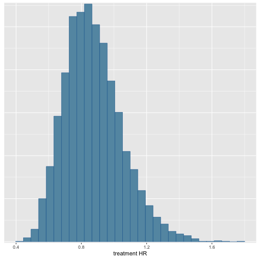
Our model does not borrow much from the external arm! This is the desired outcome given how different the control arms were.
Control arm imbalances
Check balance between arms
table1(
  ~ cov1 + cov2 + cov3 + cov4 |
    factor(ext, labels = c("Internal RCT", "External data")) +
      factor(trt, labels = c("Not treated", "Treated")),
  data = example_dataframe
)
Internal RCT |
External data |
Overall |
|||
|---|---|---|---|---|---|
| Not treated (N=50) |
Treated (N=100) |
Not treated (N=350) |
Not treated (N=400) |
Treated (N=100) |
|
| cov1 | |||||
| Mean (SD) | 0.540 (0.503) | 0.630 (0.485) | 0.740 (0.439) | 0.715 (0.452) | 0.630 (0.485) |
| Median [Min, Max] | 1.00 [0, 1.00] | 1.00 [0, 1.00] | 1.00 [0, 1.00] | 1.00 [0, 1.00] | 1.00 [0, 1.00] |
| cov2 | |||||
| Mean (SD) | 0.200 (0.404) | 0.370 (0.485) | 0.500 (0.501) | 0.463 (0.499) | 0.370 (0.485) |
| Median [Min, Max] | 0 [0, 1.00] | 0 [0, 1.00] | 0.500 [0, 1.00] | 0 [0, 1.00] | 0 [0, 1.00] |
| cov3 | |||||
| Mean (SD) | 0.760 (0.431) | 0.760 (0.429) | 0.403 (0.491) | 0.448 (0.498) | 0.760 (0.429) |
| Median [Min, Max] | 1.00 [0, 1.00] | 1.00 [0, 1.00] | 0 [0, 1.00] | 0 [0, 1.00] | 1.00 [0, 1.00] |
| cov4 | |||||
| Mean (SD) | 0.420 (0.499) | 0.460 (0.501) | 0.197 (0.398) | 0.225 (0.418) | 0.460 (0.501) |
| Median [Min, Max] | 0 [0, 1.00] | 0 [0, 1.00] | 0 [0, 1.00] | 0 [0, 1.00] | 0 [0, 1.00] |
Because the imbalance may be conditional on observed covariates, let’s adjust for propensity scores in our analysis
Create a propensity score model
ps_model <- glm(ext ~ cov1 + cov2 + cov3 + cov4,
  data = example_dataframe,
  family = binomial
)
ps <- predict(ps_model, type = "response")
example_dataframe$ps <- ps
example_dataframe$ps_cat_ <- cut(
  example_dataframe$ps,
  breaks = 5,
  include.lowest = TRUE
)
levels(example_dataframe$ps_cat_) <- c(
  "ref", "low",
  "low_med", "high_med", "high"
)
Convert the data back to a matrix with dummy variables for
ps_cat_ levels
example_matrix_ps <- create_data_matrix(
  example_dataframe,
  outcome = c("time", "cnsr"),
  trt_flag_col = "trt",
  ext_flag_col = "ext",
  covariates = ~ps_cat_
)
## Call `add_covariates()` with `covariates = c("ps_cat_low", "ps_cat_low_med", "ps_cat_high_med", "ps_cat_high" ) `Propensity score analysis without borrowing
anls_ps_no_borrow <- create_analysis_obj(
  data_matrix = example_matrix_ps,
  covariates = add_covariates(
    c("ps_cat_low", "ps_cat_low_med", "ps_cat_high_med", "ps_cat_high"),
    prior_normal(0, 10000)
  ),
  outcome = outcome_surv_exponential("time", "cnsr", prior_normal(0, 10000)),
  borrowing = borrowing_none("ext"),
  treatment = treatment_details("trt", prior_normal(0, 10000))
)

res_ps_no_borrow <- mcmc_sample(
  x = anls_ps_no_borrow,
  iter_warmup = 1000,
  iter_sampling = 5000,
  chains = 1
)
draws_ps_no_borrow <- rename_draws_covariates(
  res_ps_no_borrow$draws(),
  anls_ps_no_borrow
)

summarize_draws(draws_ps_no_borrow, ~ quantile(.x, probs = c(0.025, 0.50, 0.975)))
## # A tibble: 8 × 4
## variable `2.5%` `50%` `97.5%`
## <chr> <dbl> <dbl> <dbl>
## 1 lp__ -466. -462. -459.
## 2 treatment log HR -0.732 -0.355 0.0462
## 3 baseline log hazard rate -4.73 -4.19 -3.73
## 4 ps_cat_low -0.314 0.413 1.13
## 5 ps_cat_low_med 0.436 1.01 1.58
## 6 ps_cat_high_med 1.43 2.10 2.80
## 7 ps_cat_high 2.42 3.02 3.64
## 8 treatment HR 0.481 0.701 1.05Propensity score analysis with BDB
anls_ps_bdb <- create_analysis_obj(
  data_matrix = example_matrix_ps,
  covariates = add_covariates(
    c("ps_cat_low", "ps_cat_low_med", "ps_cat_high_med", "ps_cat_high"),
    prior_normal(0, 10000)
  ),
  outcome = outcome_surv_exponential("time", "cnsr", prior_normal(0, 10000)),
  borrowing = borrowing_hierarchical_commensurate("ext", prior_gamma(0.001, 0.001)),
  treatment = treatment_details("trt", prior_normal(0, 10000))
)

res_ps_bdb <- mcmc_sample(
  x = anls_ps_bdb,
  iter_warmup = 1000,
  iter_sampling = 5000,
  chains = 1
)
draws_ps_bdb <- rename_draws_covariates(
  res_ps_bdb$draws(),
  anls_ps_bdb
)

summarize_draws(draws_ps_bdb, ~ quantile(.x, probs = c(0.025, 0.50, 0.975)))
## # A tibble: 10 × 4
## variable `2.5%` `50%` `97.5%`
## <chr> <dbl> <dbl> <dbl>
## 1 lp__ -1426. -1421. -1418.
## 2 treatment log HR -0.702 -0.355 -0.0330
## 3 baseline log hazard rate, internal -4.65 -4.17 -3.75
## 4 baseline log hazard rate, external -4.66 -4.19 -3.77
## 5 commensurability parameter 0.119 54.3 1212.
## 6 ps_cat_low -0.364 0.250 0.853
## 7 ps_cat_low_med 0.589 1.04 1.56
## 8 ps_cat_high_med 1.62 2.08 2.59
## 9 ps_cat_high 2.51 2.93 3.43
## 10 treatment HR 0.496 0.701 0.968It looks like PS + BDB allowed us to most accurately recover the true hazard ratio of 0.70.