6. Walkthrough overview slides

Introducing `psborrow2`

Presentation flow

Bayesian Dynamic Borrowing
History of psborrow2
Overview of package
Demonstration of a single dataset analysis
Demonstration of a simulation study analysis
Installing psborrow2

Acknowledgements

psborrow2 is the culmination of work from many individuals within industry, academia, and the FDA. The below list of authors and collaborators has been integral to the package development (alphabetical):

Craig Gower-Page
Isaac Gravestock
Yichen Lu
Herb Pang
Daniel Sabanes Bove
Matthew Secrest
Jiawen Zhu

Bayesian Dynamic Borrowing

Hybrid controls

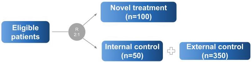
Hybrid control studies are those in which external data are used to supplement the control arm of a randomized, controlled trial (RCT). The schematic below describes such a scenario:

Types of borrowing

How best should we incorporate the knowledge we have on the external control arm?

There are several ways to do this. psborrow2 allows for three ways of incorporating external data:

Borrowing type	Description
No borrowing	Only include the internal RCT date (i.e., ignoring external controls)
Full borrowing	Pool external and internal controls
Bayesian dynamic borrowing (BDB)	Borrowing external controls to the extent that the outcomes are similar

Standard Bayesian analysis without borrowing

Consider a standard Bayesian model with survival as an endpoint without external data. This is equally valid in “No borrowing” and “Full borrowing” approaches. There are two parameters of interest:

\(\rho_{00}\), the hazard rate for the internal control
\(\rho_{10}\), the hazard rate for the internal experimental

The hazard ratio, \(\theta\), is therefore: \[ \theta = \frac{\rho_{10}}{\rho_{00}} \]

And the posterior distribution of \(\theta\) is:

\[ P(\theta | X) \propto P(X | \theta) \times P(\theta) \]

Bayesian Dynamic Borrowing

In BDB, we introduce two more parameters:

\(\rho_{01}\), the hazard rate of the external control cohort
\(\tau\), a precision parameter known as the “commensurability parameter”

Information from \(\rho_{01}\) is used in estimating \(\rho_{00}\) through a hierarchical model:

\[ \rho_{00} | \rho_{01} \sim \operatorname{Normal}\left(\rho_{01}, \frac{1}{\tau}\right) \]

The posterior distribution for \(\theta\) is then:

\[ P(\theta, \tau | X) \propto P(X | \theta, \tau) \times P(\theta | \tau) \times P(\tau) \]

Impact of \(\tau\)

The commensurability parameter, \(\tau\) dictates the extent of borrowing. This is estimated by the model but can be influenced by the choice of hyperprior. As \(\tau\) approaches infinity, the prior distribution on \(\rho_{00}\) effectively becomes \(\rho_{01}\):

\[ \rho_{00} \sim \rho_{01} \approxeq \operatorname{Normal}\left(\rho_{01}, \infty\right) \]

Choice of hyperprior for \(\tau\)

Consider two hyperprior distributions for \(\tau\):

> Warning:  [1m [22mUsing `size` aesthetic for lines was deprecated in ggplot2 3.4.0.
>  [36mℹ [39m Please use `linewidth` instead.
>  [90mThis warning is displayed once every 8 hours. [39m
>  [90mCall `lifecycle::last_lifecycle_warnings()` to see where this warning was [39m
>  [90mgenerated. [39m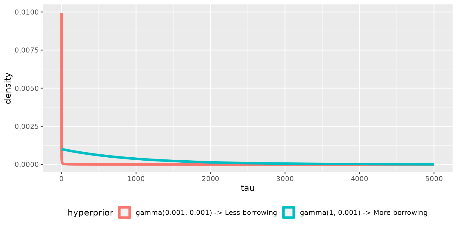

The \(gamma(1, .001)\) will induce more borrowing.

History of `psborrow2`

`psborrow2` timeline

psborrow2 is the successor to psborrow, an R package for simulation studies to aid trial design and understand the benefits of BDB on operating characteristics.

Date	Event
2019	psborrow development started
Q2 2021	CRAN v0.1.0 published
2021	Initial user feedback received from the interial POC study and the FDA CID pilot project
Q1 2022	We start a collaboration with Roche statistical engineering team to productionize the package
May 2022	psborrow v0.2.0 published (bug fixed, documentation improved) on CRAN
Jul 2022	psborrow2 development started (faster, improved UI, tests, flexibility, more outcomes)
Oct 2022	psborrow2 package made public

Overview of package

Package objectives

psborrow2 has two objectives:

1) Facilitate BDB analyses

psborrow2 has a user-friendly interface for conducting BDB analyses that handles the computationally-difficult MCMC sampling for the user

2) Facilitate simulation studies of BDB

psborrow2 can be used to compare different trial and BDB characteristics in a unified way in simulation studies to inform trial design

Demonstration of a single BDB analysis

Prior distributions

In psborrow2, the user creates fully parametric Bayesian models with proper prior distributions using the constructors:

bernoulli_prior()
beta_prior()
cauchy_prior()
exponential_prior()
gamma_prior()
normal_prior()
poisson_prior()
uniform_prior()

is(normal_prior(mu = 0, sigma = 100), "Prior")
> [1] TRUE

Plotting priors

Each Prior object has a plot method.

plot(
  normal_prior(mu = 0, sigma = 10),
  xlim = c(-100, 100),
  ylim = c(0, 0.1)
)

Plotting an uninformative normal prior

plot(
  normal_prior(mu = 0, sigma = 10000),
  xlim = c(-100, 100),
  ylim = c(0, 0.1)
)

Hyperpriors for commensurability parameters

Let’s look at a conservative hyperprior that will not encourage borrowing:

plot(
  gamma_prior(alpha = 0.001, beta = 0.001),
  xlim = c(-1, 20),
  ylim = c(0, .025)
)

Now let’s look at a more aggressive hyperprior that may induce borrowing:

plot(
  gamma_prior(alpha = 1, beta = 0.001),
  xlim = c(-1, 20),
  ylim = c(0, .025)
)

Example data

psborrow2 has simulated example data we can use in an analysis.

head(example_matrix[, c("ext", "trt", "time", "cnsr")])
>      ext trt       time cnsr
> [1,]   0   0  2.4226411    0
> [2,]   0   0 50.0000000    1
> [3,]   0   0  0.9674372    0
> [4,]   0   0 14.5774738    0
> [5,]   0   0 50.0000000    1
> [6,]   0   0 50.0000000    1

ext = 1 for external trial patients, else ext = 0
trt = 1 for experimentally-treated patients, else trt = 0
time is the time to event or censorship
cnsr = 1 if a patient’s follow-up was censored, else csnr = 0

The flags in this data.frame are explained in greater detail in ?example_matrix.

	External trial data flag		Total
	0	1	Total
Experimental treatment flag
0	50	350	400
1	100	0	100
Total	150	350	500

It looks like we have 50 patients in our internal control, 100 in our internal experimental, and 350 in our external control.

Naive internal comparisons

Let’s start by exploring the three arms descriptively:

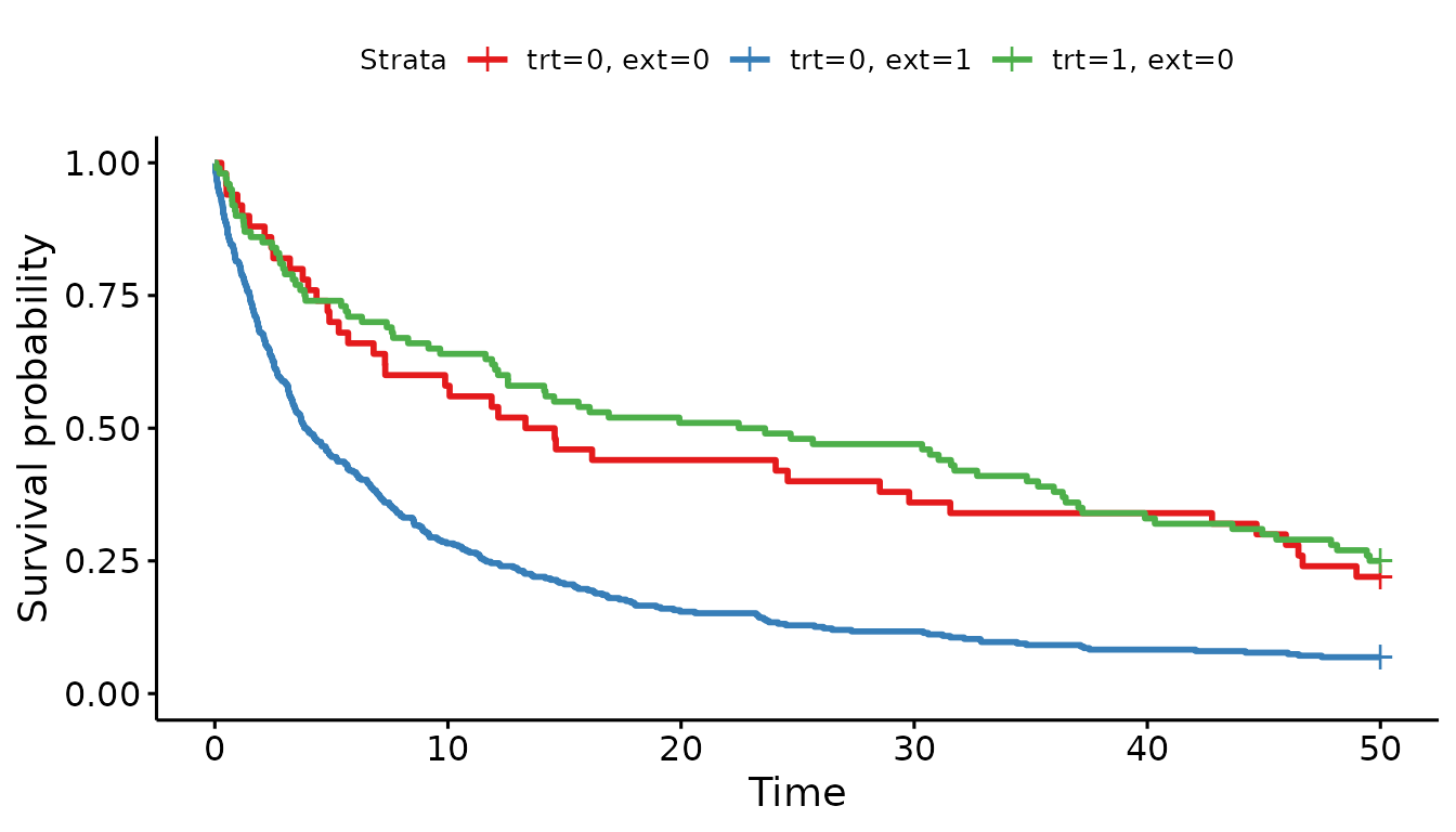
Wow, the external control population looks quite different from the internal control population!

As a point of reference, let’s conduct a Cox proportional hazards model looking just at the internal RCT data.

term	estimate	std.error	statistic	p.value	conf.low	conf.high
trt	0.90	0.20	−0.56	0.58	0.61	1.32

Here, the hazard ratio is 0.90 (95% CI 0.61 - 1.32), ignoring the external control data.

Hybrid control analysis

Let’s confirm that BDB will not perform much borrowing when we include the external data. For a BDB analysis in psborrow2, we want to create an object of class Analysis with:

create_analysis_obj(
  data_matrix,
  outcome,
  borrowing,
  treatment
)

Argument	Description
data_matrix	The data matrix, including all relevant outcome variables,and treatment arm and external control arm flags.
outcome	Object of class Outcome as output by exp_surv_dist(), weib_ph_surv_dist(), or logistic_bin_outcome().
borrowing	Object of class Borrowing as output by borrowing_details().
treatment	Object of class Treatment as output by treatment_details().

Outcome class

Let’s look at the Outcome class. There are three different outcomes supported by psborrow2, each of which has a constructor:

Constructor	Description
exp_surv_dist()	Exponential survival distribution
weib_ph_surv_dist()	Weibull survival distribution (proportional hazards formulation)
logistic_bin_outcome()	Bernoulli distribution with logit parametrization

Arguments to `exp_surv_dist()`

exp_surv_dist(
  time_var,
  cens_var,
  baseline_prior
)

The first two arguments to exp_surv_dist() are straightforward:

time_var, Name of time variable column in model matrix
cens_var, Name of the censorship variable flag in model matrix

The final argument is more complicated:

baseline_prior, Prior distribution for the log hazard rate of the external control arm.

Let’s create our outcome object with exp_surv_dist() using an uninformative Normal prior distribution for the log hazard rate of the external control arm.

exp_outcome <- exp_surv_dist(
  time_var = "time",
  cens_var = "cnsr",
  baseline_prior = normal_prior(0, 10000)
)

class(exp_outcome)
> [1] "ExponentialSurvDist"
> attr(,"package")
> [1] "psborrow2"

is(exp_outcome, "Outcome")
> [1] TRUE

Borrowing class

Borrowing class objects are created with borrowing_details().

borrowing_details(
  method,
  ext_flag_col,
  tau_prior
)

method, The type of borrowing to perform. It must be one of: 'BDB', 'Full borrowing', or 'No borrowing'
ext_flag_col, The name of the column in the data matrix that corresponds to the external control flag
tau_prior, the hyperprior for the commensurability parameter (only necessary for ‘BDB’)

Let’s create a Borrowing object with a conservative inverse Gamma distribution with rate and scale of 0.001:

bdb_borrowing <- borrowing_details(
  method = "BDB",
  ext_flag_col = "ext",
  tau_prior = gamma_prior(alpha = 0.001, beta = 0.001)
)

class(bdb_borrowing)
> [1] "Borrowing"
> attr(,"package")
> [1] "psborrow2"

Treatment class

Finally, we’ll create an object of class Treatment through the constructor treatment_details.

treatment_details(
  trt_flag_col,
  trt_prior
)

trt_flag_col, The name of the column in the model matrix that corresponds to the treatment flag
trt_prior, Object of class Prior specifying the prior distribution of the log hazard ratio for the experimental treatment

Let’s assume an uninformative prior distribution for the log hazard ratio of treatment and create our Treatment object:

trt_details <- treatment_details(
  trt_flag_col = "trt",
  trt_prior = normal_prior(0, 10000)
)

class(trt_details)
> [1] "Treatment"
> attr(,"package")
> [1] "psborrow2"

Analysis class object

Now we have all the information we need to create an object of class Analysis:

analysis_object <- create_analysis_obj(
  data_matrix = example_matrix,
  outcome = exp_outcome,
  borrowing = bdb_borrowing,
  treatment = trt_details
)

class(analysis_object)
> [1] "Analysis"
> attr(,"package")
> [1] "psborrow2"

We can do this in one function call as well:

analysis_object <- create_analysis_obj(
  data_matrix = example_matrix,
  outcome = exp_surv_dist(
    time_var = "time",
    cens_var = "cnsr",
    baseline_prior = normal_prior(0, 10000)
  ),
  borrowing = borrowing_details(
    method = "BDB",
    ext_flag_col = "ext",
    tau_prior = gamma_prior(alpha = 0.001, beta = 0.001)
  ),
  treatment = treatment_details(
    trt_flag_col = "trt",
    trt_prior = normal_prior(0, 10000)
  )
)

print(analysis_object)
> Analysis Object
> 
> Outcome model: ExponentialSurvDist 
> Outcome variables: time cnsr 
> 
> Borrowing method: BDB 
> External flag: ext 
> 
> Treatment variable: trt 
> 
> Data: Matrix with 500 observations 
>     -  50  internal controls
>     -  350  external controls 
>     -  100  internal experimental
> 
> Stan model compiled and ready to sample.
>  Call mcmc_sample() next.

Sampling from an analysis object

The Analysis object suggests calling mcmc_sample() as a next step. We’ll follow that advice!

results <- mcmc_sample(
  analysis_object,
  iter_warmup = 1000,
  iter_sampling = 1000,
  chains = 1
)

results
>  variable     mean   median   sd  mad       q5      q95 rhat ess_bulk ess_tail
>  lp__     -1618.00 -1617.66 1.63 1.39 -1621.25 -1616.15 1.00      286      408
>  beta_trt    -0.16    -0.17 0.20 0.20    -0.48     0.18 1.01      462      494
>  tau          1.14     0.44 1.95 0.62     0.00     4.81 1.00      223      224
>  alpha[1]    -3.35    -3.35 0.16 0.16    -3.63    -3.10 1.01      448      465
>  alpha[2]    -2.40    -2.40 0.06 0.05    -2.50    -2.30 1.00      684      581
>  HR_trt       0.87     0.84 0.18 0.16     0.62     1.20 1.01      462      494

At this point in our analysis, we should refer to the cmdstanr site for methods.

Let’s look at a summary of the median and 95% credible intervals:

variable	2.5%	50%	97.5%
treatment log HR	−0.54	−0.17	0.24
commensurability parameter	0.00	0.44	6.16
baseline log hazard rate, internal	−3.70	−3.35	−3.06
baseline log hazard rate, external	−2.51	−2.40	−2.29
treatment HR	0.58	0.84	1.27

Our results did not change substantially after using BDB. This is exactly what we would expect given how different our populations are!

Let’s explore baseline characteristics and see if we can identify ways in which the internal and external control arms differ:

	Control		Treatment	Overall
	Internal (N=50)	External (N=350)	Internal (N=100)	Internal (N=150)	External (N=350)
cov1
Mean (SD)	0.540 (0.503)	0.740 (0.439)	0.630 (0.485)	0.600 (0.492)	0.740 (0.439)
Median [Min, Max]	1.00 [0, 1.00]	1.00 [0, 1.00]	1.00 [0, 1.00]	1.00 [0, 1.00]	1.00 [0, 1.00]
cov2
Mean (SD)	0.200 (0.404)	0.500 (0.501)	0.370 (0.485)	0.313 (0.465)	0.500 (0.501)
Median [Min, Max]	0 [0, 1.00]	0.500 [0, 1.00]	0 [0, 1.00]	0 [0, 1.00]	0.500 [0, 1.00]
cov3
Mean (SD)	0.760 (0.431)	0.403 (0.491)	0.760 (0.429)	0.760 (0.429)	0.403 (0.491)
Median [Min, Max]	1.00 [0, 1.00]	0 [0, 1.00]	1.00 [0, 1.00]	1.00 [0, 1.00]	0 [0, 1.00]
cov4
Mean (SD)	0.420 (0.499)	0.197 (0.398)	0.460 (0.501)	0.447 (0.499)	0.197 (0.398)
Median [Min, Max]	0 [0, 1.00]	0 [0, 1.00]	0 [0, 1.00]	0 [0, 1.00]	0 [0, 1.00]

There appear to be some differences. Let’s use statistical adjustment base on the propensity score to address this:

ps_model <- glm(ext ~ cov1 + cov2 + cov3 + cov4,
  data = example_dataframe,
  family = binomial
)

ps_model
> 
> Call:  glm(formula = ext ~ cov1 + cov2 + cov3 + cov4, family = binomial, 
>     data = example_dataframe)
> 
> Coefficients:
> (Intercept)         cov1         cov2         cov3         cov4  
>      1.4389       0.5840       0.7643      -1.5827      -1.1420  
> 
> Degrees of Freedom: 499 Total (i.e. Null);  495 Residual
> Null Deviance:        610.9 
> Residual Deviance: 508.1  AIC: 518.1

We’ll make a new matrix called example_matrix_ps which has 5 categories of propensity score levels with approximately the same number of patients in each.

head(example_matrix_ps)
>         time cnsr trt ext ps_cat_low ps_cat_low_med ps_cat_high_med ps_cat_high
> 1  2.4226411    0   0   0          1              0               0           0
> 2 50.0000000    1   0   0          0              0               0           0
> 3  0.9674372    0   0   0          0              0               0           1
> 4 14.5774738    0   0   0          0              0               0           0
> 5 50.0000000    1   0   0          0              0               0           0
> 6 50.0000000    1   0   0          0              0               0           0

Adjusting for covariates in `psborrow2`

To adjust for covariates, we’ll use the costructor add_covariates():

add_covariates(
  covariates,
  priors
)

covariates, Names of columns in the data matrix containing covariates to be adjusted for
priors, Either a single object of class Prior specifying the prior distribution to apply to all covariates or a named list of distributions of class Prior, one for each covariate

Analysis object adjusting for propensity scores

Now let’s create an Analysis object that adjusts for propensity scores:

analysis_object_ps <- create_analysis_obj(
  data_matrix = example_matrix_ps,
  covariates = add_covariates(
    c("ps_cat_low", "ps_cat_low_med", "ps_cat_high_med", "ps_cat_high"),
    normal_prior(0, 10000)
  ),
  outcome = exp_surv_dist("time", "cnsr", normal_prior(0, 10000)),
  borrowing = borrowing_details("BDB", "ext", gamma_prior(0.001, 0.001)),
  treatment = treatment_details("trt", normal_prior(0, 10000))
)

results_ps <- mcmc_sample(analysis_object_ps,
  iter_warmup = 1000,
  iter_sampling = 1000,
  chains = 1
)

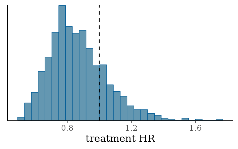
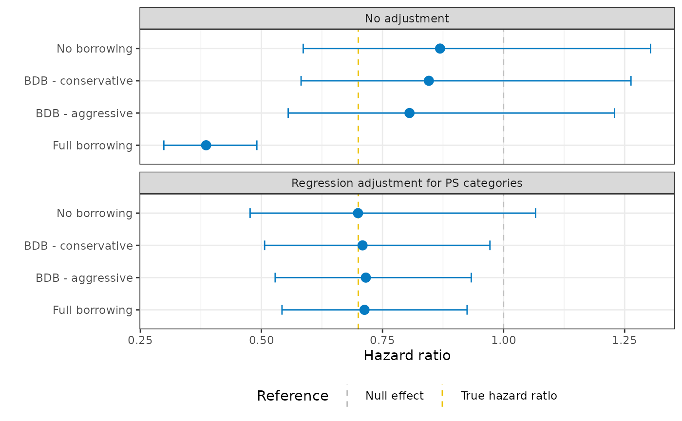
It looks like we do indeed see a treatment effect when differences in the distributions of baseline confounds are taken into consideration!

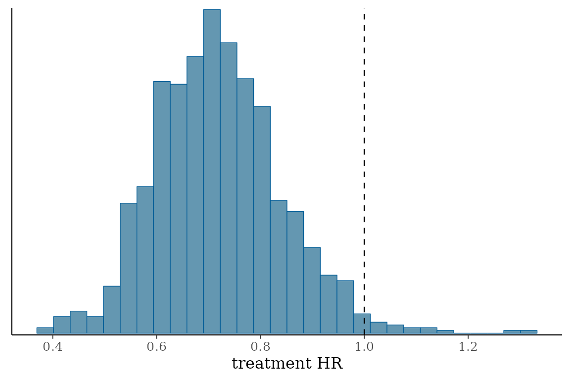
variable	2.5%	50%	97.5%
treatment log HR	−0.68	−0.34	−0.03
commensurability parameter	0.27	57.48	1,391.63
baseline log hazard rate, internal	−4.73	−4.18	−3.76
baseline log hazard rate, external	−4.72	−4.20	−3.79
ps_cat_low	−0.30	0.27	0.84
ps_cat_low_med	0.62	1.06	1.58
ps_cat_high_med	1.64	2.11	2.65
ps_cat_high	2.52	2.94	3.46
treatment HR	0.51	0.71	0.97

The histogram of MCMC samples confirms this as well:

Summary of analyses

Demonstration of a simulation study

Simulation study

We now turn to the question of how to design trials with BDB in mind. Here, we will create an object of class Simulation with create_simulation_obj():

create_simulation_obj(
  data_matrix_list,
  outcome,
  borrowing,
  treatment
)

If this looks similar to create_analysis_obj(), that is by design!

`sim_data_list()`

The first argument we need to fill in is data_matrix_list, created with sim_data_list().

sim_data_list(
  data_list,
  guide,
  effect,
  drift,
  index
)

The first argument is a list of lists of matrices. At the highest level, we’ll index different data generation parameters. At the lowest level, we’ll index different matrices generated with these parameters.

`data_list`

This example data_list object is a list of lists with two data generation scenarios (e.g., true HR of 1.0 and true HR of 0.8).

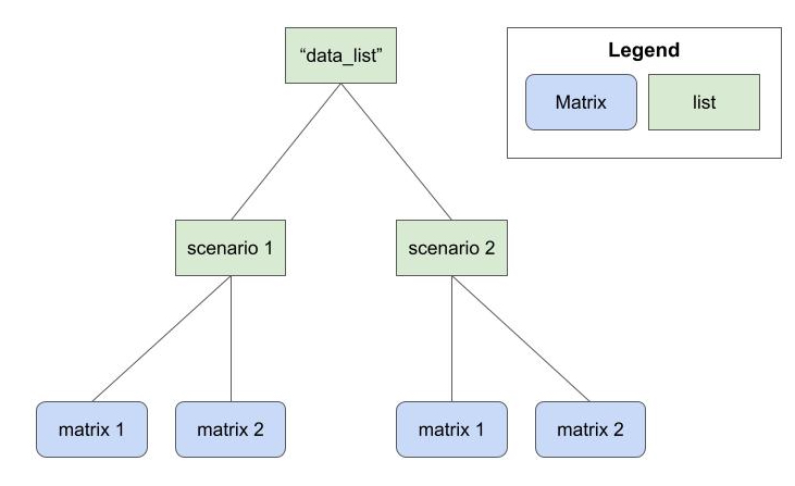
Suppose we have a list of lists of simulated data called my_data_list:

There are four scenarios.

NROW(my_data_list)
> [1] 4

Each scenario has 100 matrices.

NROW(my_data_list[[1]])
> [1] 100

head(my_data_list[[1]][[1]], 3)
>      id ext trt     time status cnsr
> [1,]  1   0   0 8.179722      1    0
> [2,]  2   0   0 6.884286      1    0
> [3,]  3   0   0 2.348331      1    0

Data generation guide

We also need to create a guide that explains how the data were generated. In this example, the four scenarios are summarized with the below guide:

my_sim_data_guide
>   true_hr          drift_hr id
> 1     0.6       No drift HR  1
> 2     1.0       No drift HR  2
> 3     0.6 Moderate drift HR  3
> 4     1.0 Moderate drift HR  4

This guide implies that my_sim_data_guide[[1]] is a list of matrices where the treatment HR was 0.6 and the drift HR was 1.0.

Finally, we need to specify where in the guide three important features are: the true hazard ratio, the drift hazard ratio, and the index. These are all the columns we have in our guide, so we simply specify the column names:

my_sim_data_list <- sim_data_list(
  data_list = my_data_list,
  guide = my_sim_data_guide,
  effect = "true_hr",
  drift = "drift_hr",
  index = "id"
)

my_sim_data_list
> SimDataList object with  4  different scenarios
>   true_hr          drift_hr id n_datasets_per_param
> 1     0.6       No drift HR  1                  100
> 2     1.0       No drift HR  2                  100
> 3     0.6 Moderate drift HR  3                  100
> 4     1.0 Moderate drift HR  4                  100

Borrowing list

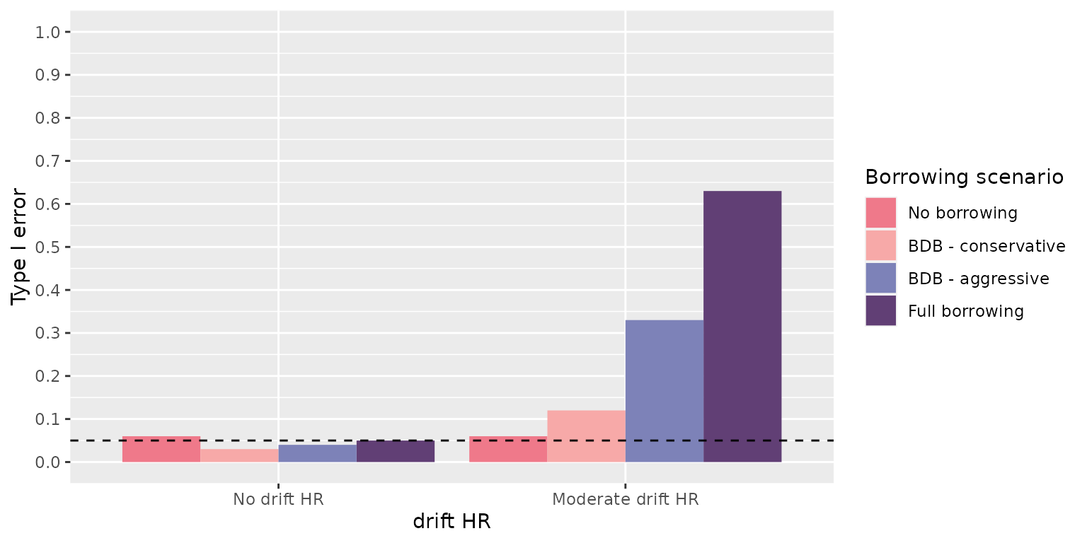
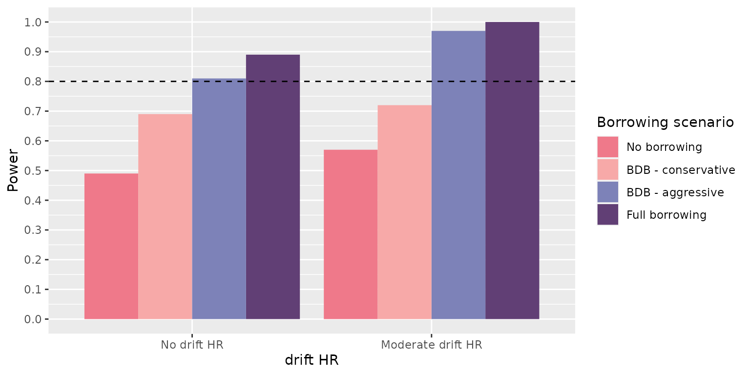
For this simulation study, let’s focus on comparing four borrowing methods:

No borrowing
BDB, conservative hyperprior
BDB, aggressive hyperprior
Full borrowing

How do we specify that we want to evaluate multiple borrowing methods? We’ll use a special list of Borrowing objects, which we’ll create through the function sim_borrowing_list().

sim_borrowing_list() needs a named list of Borrowing objects:

my_borrowing_list <- sim_borrowing_list(
  list(
    "No borrowing" = borrowing_details("No borrowing", "ext"),
    "Full borrowing" = borrowing_details("Full borrowing", "ext"),
    "BDB - conservative" = borrowing_details("BDB", "ext", gamma_prior(0.001, 0.001)),
    "BDB - aggressive" = borrowing_details("BDB", "ext", gamma_prior(1, 0.001))
  )
)

my_borrowing_list
> SimBorrowingList object with  4  different scenario(s)
>   borrowing_scenario
> 1       No borrowing
> 2     Full borrowing
> 3 BDB - conservative
> 4   BDB - aggressive

Note, in this example we’ll only pass a list of Borrowing objects, but similar constructors exist for other psborrow2 objects:

sim_treatment_list()
sim_covariate_list()
sim_outcome_list()

Note: If you do not want to vary parameters in your simulation study, you can simply pass an unlisted object. That is, you could call borrowing_details() instead of sim_borrowing_list().

`create_simulation_obj()`

Now, let’s create a Simulation object:

simulation_obj <- create_simulation_obj(
  my_sim_data_list,
  outcome = exp_surv_dist("time",
    "cnsr",
    baseline_prior = normal_prior(0, 10000)
  ),
  borrowing = my_borrowing_list,
  treatment = treatment_details(
    trt_flag_col = "trt",
    trt_prior = normal_prior(0, 10000)
  )
)

`mcmc_sample()`

As with Analysis objects, the next step for us with Simulation objects is to call mcmc_sample():

simulation_res <- mcmc_sample(
  simulation_obj,
  iter_warmup = 1000,
  iter_sampling = 1000,
  chains = 1
)

You’ll note the simulation study results are a special psborrow2 class, NOT a CmdStanMCMC object (as with Analysis objects).

simulation_res
> `MCMCSimulationResult` object.  Call `get_results()` to save outputs as a data.frame

Let’s get a useful data.frame of results by calling get_results:

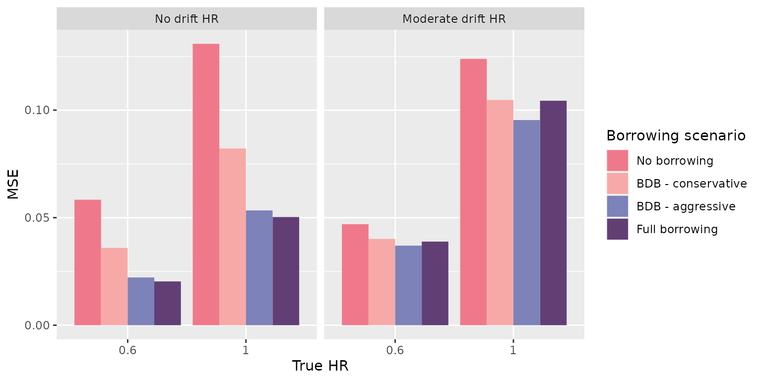
simulation_res_df <- get_results(simulation_res)

Simulation study results

Let’s see what exactly is contained in the results.

colnames(simulation_res_df)
>  [1] "true_hr"              "drift_hr"             "id"                  
>  [4] "n_datasets_per_param" "outcome_scenario"     "borrowing_scenario"  
>  [7] "covariate_scenario"   "treatment_scenario"   "mse_mean"            
> [10] "bias_mean"            "null_coverage"        "true_coverage"

mse_mean, the mean MSE for results
bias_mean, the mean bias for the results
null_coverage, the proportion of results that contain the null effect (1.0) in the specified credible interval quantiles (default are 0.025 - 0.975)
true_coverage, the proportion of results that contain the true effect in the specified credible interval quantiles (default are 0.025 - 0.975)

Let’s look at the number of parameter combinations that were evaluated:

NROW(simulation_res_df)
> [1] 16

head(simulation_res_df, 2)
>   true_hr    drift_hr id n_datasets_per_param outcome_scenario
> 1     0.6 No drift HR  1                  100          default
> 2     1.0 No drift HR  2                  100          default
>   borrowing_scenario covariate_scenario treatment_scenario   mse_mean
> 1       No borrowing      No adjustment            default 0.05834557
> 2       No borrowing      No adjustment            default 0.13082015
>    bias_mean null_coverage true_coverage
> 1 0.05878194          0.51          0.97
> 2 0.03238762          0.94          0.94

This makes sense as we had 4 scenarios in our data generation step and 4 in our borrowing step. The cartesian product is 16.

MSE

We can use the results to plot MSE by scenario as below:

Type I error

Because we included a true HR of 1.0, we can evaluate type I error by looking at the compliment to the true parameter coverage:

Power

We can include power by looking at the results for our true simulation of 0.6.

Installing `psborrow2`

psborrow2 can be installed from GitHub with:

devtools::install_git("https://github.com/Genentech/psborrow2")

Feedback can be provided through GitHub issues:

https://github.com/Genentech/psborrow2/issues

The vignettes can be accessed with:

browseVignettes("psborrow2")

Matt Secrest

Introducing psborrow2

Presentation flow

Acknowledgements

Bayesian Dynamic Borrowing

Hybrid controls

Types of borrowing

Standard Bayesian analysis without borrowing

Bayesian Dynamic Borrowing

Impact of \(\tau\)

Choice of hyperprior for \(\tau\)

History of psborrow2

psborrow2 timeline

Overview of package

Package objectives

1) Facilitate BDB analyses

2) Facilitate simulation studies of BDB

Demonstration of a single BDB analysis

Prior distributions

Plotting priors

Plotting an uninformative normal prior

Hyperpriors for commensurability parameters

Example data

Naive internal comparisons

Hybrid control analysis

Outcome class

Arguments to exp_surv_dist()

Borrowing class

Treatment class

Analysis class object

Sampling from an analysis object

Adjusting for covariates in psborrow2

Analysis object adjusting for propensity scores

Summary of analyses

Demonstration of a simulation study

Simulation study

sim_data_list()

data_list

Data generation guide

Borrowing list

create_simulation_obj()

mcmc_sample()

Simulation study results

MSE

Type I error

Power

Installing psborrow2

Thank you!

Introducing `psborrow2`

History of `psborrow2`

`psborrow2` timeline

Arguments to `exp_surv_dist()`

Adjusting for covariates in `psborrow2`

`sim_data_list()`

`data_list`

`create_simulation_obj()`

`mcmc_sample()`

Installing `psborrow2`