4. Conduct a simulation study

In this vignette, you’ll learn how to use psborrow2 to create a simulation study with the goal of informing trial design. Let’s load psborrow2 to start:

library(psborrow2)

Bringing your own simulated data

We’ll start by showing how to conduct a simulation study when you bring your own simulated data. To execute a simulation study with your own data, we need to build an object of class Simulation using the function create_simulation_obj(). Let’s look at the arguments to create_simulation_obj() and consider them one-by-one below:

create_simulation_obj(
  data_matrix_list,
  outcome,
  borrowing,
  covariate,
  treatment
)

`data_matrix_list`

data_matrix_list is where you input the data you will be using for the simulation study using the function sim_data_list().

The first argument is a list of lists of matrices. At the highest level, we’ll index different data generation parameters. At the lowest level, we’ll index different matrices generated with these parameters.

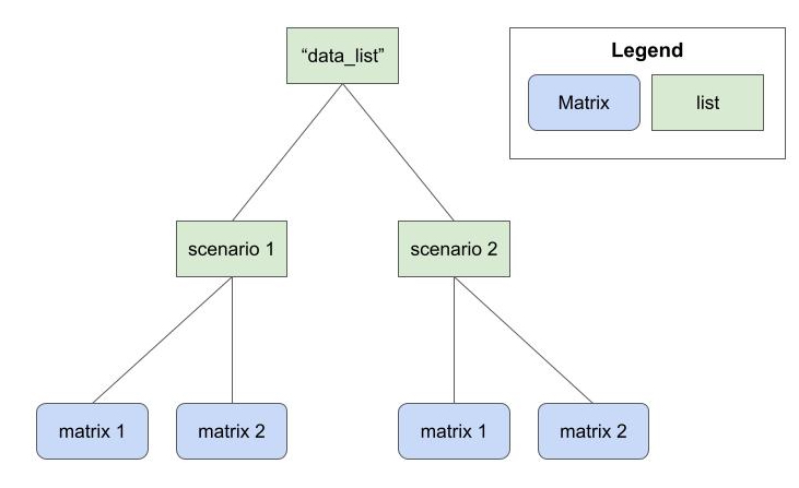
`data_list`

Figure 1 below depicts an example data_list object. This object is a list of lists with two data generation scenarios (e.g., true HR of 1.0 and true HR of 0.8). Each scenario is arranged as a list of matrices that were generated according to that data generation scenario.

Figure 1

We’ll use the simsurv package to generate survival data and we’ll then put it in a similar format. In this example, we’ll vary two data generation parameters: true HR and drift HR (the HR comparing external to internal controls). Suppose we have a function, sim_single_matrix() which can simulate data for a single matrix.

That is:

library(simsurv)
# function to create a single matrix
sim_single_matrix <- function(n = 500, # n simulated pts
                              prob = c(
                                0.1, # proportion internal control
                                0.2, # proportion internal treated
                                0.7
                              ), # proportion external control
                              hr = 0.70, # true HR for the treatment
                              drift_hr = 1.0 # HR of external/internal
) {
  # checks
  if (sum(prob) != 1.0) {
    stop("prob must sum to 1")
  }

  # data frame with the subject IDs and treatment group
  df_ids <- data.frame(
    id = 1:n,
    ext = c(
      rep(0L, n * (prob[1] + prob[2])),
      rep(1L, n * prob[3])
    ),
    trt = c(
      rep(0L, n * prob[1]),
      rep(1L, n * prob[2]),
      rep(0L, n * prob[3])
    )
  )

  # simulated event times
  df_surv <- simsurv(
    lambdas = 0.1,
    dist = "exponential",
    betas = c(
      trt = log(hr),
      ext = log(drift_hr)
    ),
    x = df_ids,
    maxt = 50
  )

  df_surv$censor <- 1 - df_surv$status

  # merge the simulated event times into data frame
  df <- merge(df_ids, df_surv)
  df <- df[, c("id", "ext", "trt", "eventtime", "status", "censor")]
  colnames(df) <- c("id", "ext", "trt", "time", "status", "cnsr")
  return(as.matrix(df))
}

head(sim_single_matrix(n = 500, hr = 0.5, drift_hr = 1.2))
#      id ext trt       time status cnsr
# [1,]  1   0   0  7.4973598      1    0
# [2,]  2   0   0  7.4607791      1    0
# [3,]  3   0   0  0.2433736      1    0
# [4,]  4   0   0  5.5029255      1    0
# [5,]  5   0   0  3.7491904      1    0
# [6,]  6   0   0 16.9655617      1    0

Using this function, let’s simulate a list of lists of matrices with four scenarios:

True HR = 0.6, drift HR = 1.0
True HR = 1.0, drift HR = 1.0
True HR = 0.6, drift HR = 1.5
True HR = 1.0, drift HR = 1.5

# Seed for reproducibility
set.seed(123)

# Number of simulations per scenario
n <- 100

# Create list of lists of data
my_data_list <- list(
  replicate(n,
    sim_single_matrix(n = 250, hr = 0.6, drift_hr = 1.0),
    simplify = FALSE
  ),
  replicate(n,
    sim_single_matrix(n = 250, hr = 1.0, drift_hr = 1.0),
    simplify = FALSE
  ),
  replicate(n,
    sim_single_matrix(n = 250, hr = 0.6, drift_hr = 1.5),
    simplify = FALSE
  ),
  replicate(n,
    sim_single_matrix(n = 250, hr = 1.0, drift_hr = 1.5),
    simplify = FALSE
  )
)

There are 4 scenarios.

NROW(my_data_list)
# [1] 4

Each scenario has 100 matrices.

NROW(my_data_list[[1]])
# [1] 100

The lowest level of the list of lists is a data matrix.

head(my_data_list[[1]][[1]])
#      id ext trt      time status cnsr
# [1,]  1   0   0  8.179722      1    0
# [2,]  2   0   0  6.884286      1    0
# [3,]  3   0   0  2.348331      1    0
# [4,]  4   0   0 17.898011      1    0
# [5,]  5   0   0  3.870353      1    0
# [6,]  6   0   0  6.795403      1    0

`guide`

In order to summarize the results from the different parameters in your simulation study, psborrow2 needs to know how the simulation parameters differ. That is the purpose of the argument guide, which is a data.frame that distinguishes the simulation study parameters. Three columns are required in guide, though many more can be provided. The three required columns are:

The true treatment effect (in our case a HR)
The true drift effect (in our case a HR). Drift effects >1 will mean that the external control arm experiences greater hazard than the internal control arm.
The name of a column that indexes the data_list

In this example, the 4 scenarios are summarized with the below guide:

my_sim_data_guide <- expand.grid(
  true_hr = c(0.6, 1.0),
  drift_hr = c("No drift HR", "Moderate drift HR")
)

my_sim_data_guide$id <- seq(1, NROW(my_sim_data_guide))

my_sim_data_guide
#   true_hr          drift_hr id
# 1     0.6       No drift HR  1
# 2     1.0       No drift HR  2
# 3     0.6 Moderate drift HR  3
# 4     1.0 Moderate drift HR  4

This guide implies that my_sim_data_guide[[1]] is a list of matrices where the treatment HR was 0.6 and the drift HR was 1.0.

`effect`, `drift`, and `index`

The last three inputs to sim_data_list(), effect, drift, and index are the column names in guide that correspond to the true treatment effect, true drift effect, and index of the data_list items, respectively. For our study, these are "true_hr", "drift_hr", and "id".

Putting it all together, we can create an object of class SimDataList:

my_sim_data_list <- sim_data_list(
  data_list = my_data_list,
  guide = my_sim_data_guide,
  effect = "true_hr",
  drift = "drift_hr",
  index = "id"
)

my_sim_data_list
# SimDataList object with  4  different scenarios
#   true_hr          drift_hr id n_datasets_per_param
# 1     0.6       No drift HR  1                  100
# 2     1.0       No drift HR  2                  100
# 3     0.6 Moderate drift HR  3                  100
# 4     1.0 Moderate drift HR  4                  100

`outcome`

outcome is where you pass information on the study outcomes. You can pass either a single Outcome class object (e.g., as produced by exp_surv_dist()), or a list of Outcome class objects passed to sim_outcome_list(). For our example, let’s just use a single exponential distribution.

my_sim_out <- exp_surv_dist(
  time_var = "time",
  cens_var = "cnsr",
  baseline_prior = normal_prior(0, 1000)
)

my_sim_out
# Outcome object with class ExponentialSurvDist 
# 
# Outcome variables:
# time_var cens_var 
#   "time"   "cnsr" 
# 
# Baseline prior:
# Normal Distribution
# Parameters:
#  Stan  R    Value
#  mu    mean    0 
#  sigma sd   1000

`borrowing`

borrowing is where we input information on the type of borrowing we want to evaluate. This can be either a single object of class Borrowing or a list of objects created with sim_borrowing_list(). For the sake of example, let’s assume we are interested in comparing four borrowing scenarios:

No borrowing
BDB, conservative hyperprior
BDB, aggressive hyperprior
Full borrowing

How do we specify that we want to evaluate multiple borrowing methods? We’ll use a special list of Borrowing objects, which we’ll create through the function sim_borrowing_list().

my_borrowing_list <- sim_borrowing_list(
  list(
    "No borrowing" = borrowing_details("No borrowing", "ext"),
    "Full borrowing" = borrowing_details("Full borrowing", "ext"),
    "BDB - conservative" = borrowing_details("BDB", "ext", gamma_prior(0.001, 0.001)),
    "BDB - aggressive" = borrowing_details("BDB", "ext", gamma_prior(1, 0.001))
  )
)

my_borrowing_list
# SimBorrowingList object with  4  different scenario(s)
#   borrowing_scenario
# 1       No borrowing
# 2     Full borrowing
# 3 BDB - conservative
# 4   BDB - aggressive

`covariate`

covariate is for information on covariate adjustment details. This can be a single instance of class Covariates from add_covariates() or a list of Covariates objects created by sim_covariate_list() . This is also the only argument that is not required in create_simulation_obj. Let’s leave this argument empty (i.e., let’s not adjust for any covariates).

`treatment`

treatment is where we input the treatment details for our simulation study. As with other inputs, this can be a single instance of a class Treatment, or a list of these classes, created with sim_treatment_list(). Let’s just use a single instance:

my_sim_treat <- treatment_details("trt", normal_prior(0, 1000))

my_sim_treat
# Treatment object
# 
# Treatment flag column: trt 
# 
# Treatment effect prior:
# Normal Distribution
# Parameters:
#  Stan  R    Value
#  mu    mean    0 
#  sigma sd   1000

`create_simulation_obj()`

Now that we have all of the relevant inputs for create_simulation_obj(), let’s call the function, which will generate and compile Stan models ready to sample on our behalf.

Important: psborrow2 will simulate the Cartesian product of all unique list elements in data_matrix_list, outcome, borrowing, covariate, and treatment. We have 4 data generation scenarios and 4 borrowing scenarios. The other inputs just have one scenario (or 0 for covariate, which is equivalent to one scenario). This means we should expect 4 \(\times\) 4 \(=\) 16 combinations of parameters. Let’s create a simulation object of class Simulation:

simulation_obj <- create_simulation_obj(
  my_sim_data_list,
  outcome = my_sim_out,
  borrowing = my_borrowing_list,
  treatment = my_sim_treat
)

simulation_obj
# Simulation object with  16  combinations and  1600  analyses ready to sample.  This is a lot of combinations/analyses! Consider breaking the  study into different simulation objects. Or if you  prefer to use these combinations, call `mcmc_sample()` next.

While we get a warning about the size of the simulation study, we are not worried because we are limiting our MCMC samples below in this example.

We can access the guide to see the specific scenarios that will be simulated with show_guide():

show_guide(simulation_obj)
#    true_hr          drift_hr id n_datasets_per_param outcome_scenario
# 1      0.6       No drift HR  1                  100          default
# 2      1.0       No drift HR  2                  100          default
# 3      0.6 Moderate drift HR  3                  100          default
# 4      1.0 Moderate drift HR  4                  100          default
# 5      0.6       No drift HR  1                  100          default
# 6      1.0       No drift HR  2                  100          default
# 7      0.6 Moderate drift HR  3                  100          default
# 8      1.0 Moderate drift HR  4                  100          default
# 9      0.6       No drift HR  1                  100          default
# 10     1.0       No drift HR  2                  100          default
# 11     0.6 Moderate drift HR  3                  100          default
# 12     1.0 Moderate drift HR  4                  100          default
# 13     0.6       No drift HR  1                  100          default
# 14     1.0       No drift HR  2                  100          default
# 15     0.6 Moderate drift HR  3                  100          default
# 16     1.0 Moderate drift HR  4                  100          default
#    borrowing_scenario covariate_scenario treatment_scenario
# 1        No borrowing      No adjustment            default
# 2        No borrowing      No adjustment            default
# 3        No borrowing      No adjustment            default
# 4        No borrowing      No adjustment            default
# 5      Full borrowing      No adjustment            default
# 6      Full borrowing      No adjustment            default
# 7      Full borrowing      No adjustment            default
# 8      Full borrowing      No adjustment            default
# 9  BDB - conservative      No adjustment            default
# 10 BDB - conservative      No adjustment            default
# 11 BDB - conservative      No adjustment            default
# 12 BDB - conservative      No adjustment            default
# 13   BDB - aggressive      No adjustment            default
# 14   BDB - aggressive      No adjustment            default
# 15   BDB - aggressive      No adjustment            default
# 16   BDB - aggressive      No adjustment            default

`mcmc_sample()`

Now that we’ve created a simulation object, we’re ready to call mcmc_sample() and generate draws for our model.

Note there is one important additional argument to mcmc_sample() for simulation objects: posterior_quantiles. This numeric vector of length 2 specifies the quantiles for null coverage and true coverage. For instance, 95% credible coverage would be estimated with posterior_quantiles = c(0.025, 0.975), the default argument.

simulation_res <- mcmc_sample(
  simulation_obj,
  posterior_quantiles = c(0.025, 0.975),
  iter_warmup = 400,
  iter_sampling = 1000,
  chains = 1L,
  seed = 112233
)

Note unlike an analysis on a single dataset, mcmc_sample() does not return a CmdStanModel object when applied to a simulation study object. Instead, it returns a class unique to simulation study results: MCMCSimulationResult.

class(simulation_res)
# [1] "MCMCSimulationResult"
# attr(,"package")
# [1] "psborrow2"

This evaluation took about 13.1 minutes. Let’s look at the performance of our simulation study by extracting the data.frame that summarizes results, get_results():

simulation_res_df <- get_results(simulation_res)
head(simulation_res_df)
#   true_hr          drift_hr id n_datasets_per_param outcome_scenario
# 1     0.6       No drift HR  1                  100          default
# 2     1.0       No drift HR  2                  100          default
# 3     0.6 Moderate drift HR  3                  100          default
# 4     1.0 Moderate drift HR  4                  100          default
# 5     0.6       No drift HR  1                  100          default
# 6     1.0       No drift HR  2                  100          default
#   borrowing_scenario covariate_scenario treatment_scenario   mse_mean
# 1       No borrowing      No adjustment            default 0.05957157
# 2       No borrowing      No adjustment            default 0.13155107
# 3       No borrowing      No adjustment            default 0.04747871
# 4       No borrowing      No adjustment            default 0.12865600
# 5     Full borrowing      No adjustment            default 0.02033351
# 6     Full borrowing      No adjustment            default 0.05067211
#    bias_mean null_coverage true_coverage
# 1 0.06379999          0.53          0.96
# 2 0.03894101          0.96          0.96
# 3 0.01517944          0.47          0.95
# 4 0.03225091          0.95          0.95
# 5 0.02193270          0.10          0.96
# 6 0.01079782          0.97          0.97

Let’s quickly visualize the results using ggplot2. We will first load ggplot2 and factorize our borrowing scenarios:

# Load ggplot2
library(ggplot2)

# Factorize
simulation_res_df$borrowing_scenario <- factor(simulation_res_df$borrowing_scenario,
  levels = c(
    "No borrowing",
    "BDB - conservative",
    "BDB - aggressive",
    "Full borrowing"
  )
)

MSE

ggplot(simulation_res_df) +
  geom_bar(aes(x = factor(true_hr), fill = borrowing_scenario, y = mse_mean),
    stat = "identity", position = "dodge"
  ) +
  labs(
    fill = "Borrowing scenario",
    x = "True HR",
    y = "MSE"
  ) +
  facet_wrap(~drift_hr) +
  scale_fill_manual(values = c("#EF798A", "#F7A9A8", "#7D82B8", "#613F75"))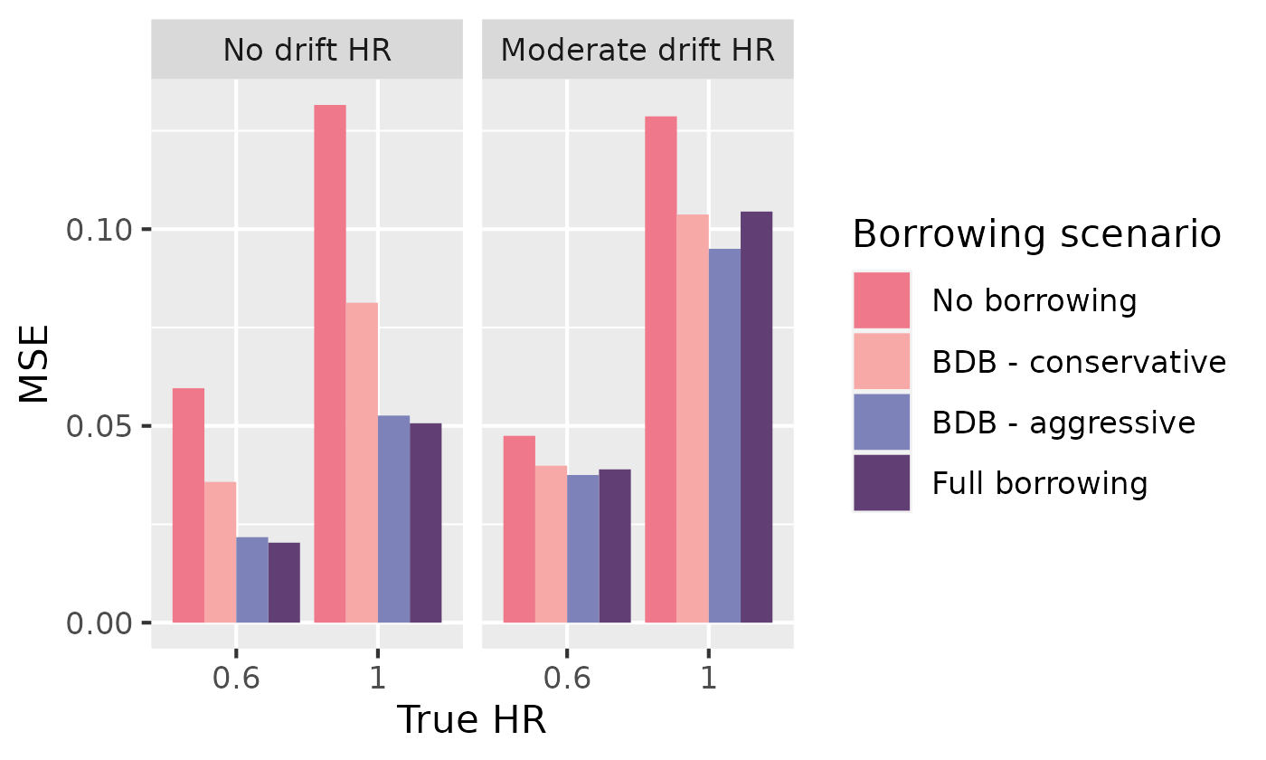

Type I error

Because we included a true HR of 1.0, we can evaluate type I error by looking at the compliment to the true parameter coverage:

ggplot(simulation_res_df[simulation_res_df$true_hr == 1.0, ]) +
  geom_bar(aes(x = factor(drift_hr), fill = borrowing_scenario, y = 1 - true_coverage),
    stat = "identity", position = "dodge"
  ) +
  labs(
    fill = "Borrowing scenario",
    x = "drift HR",
    y = "Type I error"
  ) +
  scale_fill_manual(values = c("#EF798A", "#F7A9A8", "#7D82B8", "#613F75")) +
  scale_y_continuous(breaks = seq(0, 1, .1), limits = c(0, 1)) +
  geom_hline(aes(yintercept = 0.05), linetype = 2)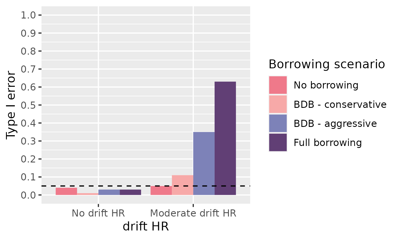

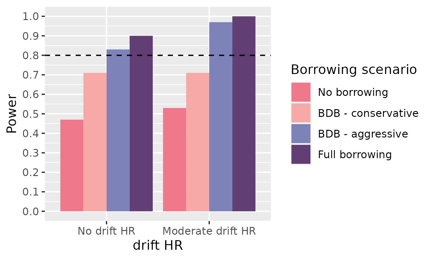
Power

We can include power by looking at the results for our true simulation of 0.6.

ggplot(simulation_res_df[simulation_res_df$true_hr == 0.6, ]) +
  geom_bar(aes(x = factor(drift_hr), fill = borrowing_scenario, y = 1 - null_coverage),
    stat = "identity", position = "dodge"
  ) +
  labs(
    fill = "Borrowing scenario",
    x = "drift HR",
    y = "Power"
  ) +
  scale_fill_manual(values = c("#EF798A", "#F7A9A8", "#7D82B8", "#613F75")) +
  scale_y_continuous(breaks = seq(0, 1, .1), limits = c(0, 1)) +
  geom_hline(aes(yintercept = 0.80), linetype = 2)

Matt Secrest and Isaac Gravestock

Bringing your own simulated data

data_matrix_list

data_list

guide

effect, drift, and index

outcome

borrowing

covariate

treatment

create_simulation_obj()

mcmc_sample()

MSE