Model Fitting

Here we describe the basic steps of joint model fitting with jmpost.

Model Specification

Each JointModel needs to be specified with three parts:

longitudinal: The model for the longitudinal outcomes.
survival: The model for the survival outcomes.
link: The link that specifies how the longitudinal model parameters enter the survival model.

Default Options

Let’s first specify a very simple joint model with:

A random slope model for the longitudinal outcome.
A Weibull proportional hazards model for the survival outcome.
The link between the two models is that the random slope from the longitudinal model enters as a product with a link coefficient into the linear predictor of the survival model.

simple_model <- JointModel(
    longitudinal = LongitudinalRandomSlope(),
    survival = SurvivalWeibullPH(),
    link = linkDSLD()
)

Note that here we use all the default options for the two models and the link, in particular the prior distributions and the initial values in the MCMC chain for the parameters are automatically chosen. We can see this from the arguments of the constructors (or from the help page):

args(LongitudinalRandomSlope)
#> function (intercept = prior_normal(30, 10), slope_mu = prior_normal(1, 
#>     3), slope_sigma = prior_lognormal(0, 1.5), sigma = prior_lognormal(0, 
#>     1.5)) 
#> NULL

So here we see that the Longitudinal Random Slope model has 4 parameters that we can define a prior for.

Specifying Priors

We can alternatively also specify the prior distributions for the parameters manually. This is important in practice to obtain a meaningful model specification and hence converging MCMC chains that allow to estimate the posterior distributions.

For the random slope model for the longitudinal outcome, we can e.g. say:

random_slope_model <- LongitudinalRandomSlope(
    intercept = prior_normal(40, 5),
    slope_mu = prior_normal(10, 2)
)

This sets the prior for the intercept to be a $N(40, 5)$ distribution and the prior for the slope_mu parameter to be a $N(10, 2)$ distribution.

Separate Models

It is also possible to not link the longitudinal and the survival models, by using the special linkNone() link specification. For example,

simple_model_no_link <- JointModel(
    longitudinal = LongitudinalRandomSlope(),
    survival = SurvivalWeibullPH(),
    link = linkNone()
)

would allow to fit the two models separately, but in the same MCMC chain.

Single Models

It is also possible to specify only the longitudinal or the survival model. Then these can be estimated on their own with separate MCMC chains.

single_longitudinal <- JointModel(
    longitudinal = LongitudinalRandomSlope()
)
single_survival <- JointModel(
    survival = SurvivalWeibullPH()
)

Data Preparation

Before we can fit the models, we need to prepare the data in the right format.

Simulating Data

Here we start from a simulated data set.

We assign 50 subjects each to the two treatment arms.
We use a time grid from 1 to 2000, e.g. specifying the days after randomization.
We use an exponentially distributed censoring time with mean of 9000 days.
We use a categorical covariate with three levels A, B and C in the overall survival model, drawn uniformly from the three levels. (Note that this is hardcoded at the moment, so the levels need to be A, B, C.)
We use another continuous covariate in the overall survival model generated from a standard normal distribution, with coefficient 0.3.
For the longitudinal outcome, we draw the values from a random slope model with the given parameters.
For the survival outcome, we draw the true value from a Weibull model. Note that it is fairly easy to put here another choice, you just need to specify a function of time returning the log baseline hazard under the given survival model.

So let’s run the code for that:

set.seed(129)
sim_data <- SimJointData(
    design = list(
        SimGroup(50, "Arm-A", "Study-X"),
        SimGroup(50, "Arm-B", "Study-X")
    ),
    longitudinal = SimLongitudinalRandomSlope(
        times = c(1, 50, 100, 150, 200, 250, 300),
        intercept = 30,
        slope_mu = c(1, 2),
        slope_sigma = 0.2,
        sigma = 20,
        link_dsld = 0.1
    ),
    survival = SimSurvivalWeibullPH(
        lambda = 1 / 300,
        gamma = 0.97,
        time_max = 2000,
        time_step = 1,
        lambda_cen = 1 / 9000,
        beta_cat = c(
            "A" = 0,
            "B" = -0.1,
            "C" = 0.5
        ),
        beta_cont = 0.3
    )
)

We might get a message here that a few subjects did not die before the day 2000, but this is not of concern. Basically it just gives us a feeling of how many survival events are included in the data set.

Formatting Data

Next we bring the data into the right format.

We start with extracting data into individual data sets, and then reducing the longitudinal data to specific time points.

os_data <- sim_data@survival
long_data <- sim_data@longitudinal

Let’s have a quick look at the format:

The survival data has:

subject ID
time point
continuous covariate value
categorical covariate level
event indicator (1 for observed, 0 for censored)
study ID
treatment arm

head(os_data)
#> # A tibble: 6 × 7
#>   subject     study   arm    time event cov_cont cov_cat
#>   <chr>       <fct>   <fct> <dbl> <dbl>    <dbl> <fct>  
#> 1 subject_001 Study-X Arm-A    35     1   -1.12  B      
#> 2 subject_002 Study-X Arm-A    17     1   -0.990 C      
#> 3 subject_003 Study-X Arm-A   876     1   -1.37  C      
#> 4 subject_004 Study-X Arm-A   100     1   -1.36  C      
#> 5 subject_005 Study-X Arm-A     9     1    2.00  B      
#> 6 subject_006 Study-X Arm-A   122     1    0.696 B

The longitudinal data has:

subject ID
time point
sum of longest diameters (SLD)
study ID
treatment arm
observation flag

head(long_data)
#> # A tibble: 6 × 6
#>   subject     arm   study    time   sld observed
#>   <chr>       <fct> <fct>   <dbl> <dbl> <lgl>   
#> 1 subject_001 Arm-A Study-X     1  23.4 TRUE    
#> 2 subject_001 Arm-A Study-X    50 108.  FALSE   
#> 3 subject_001 Arm-A Study-X   100 137.  FALSE   
#> 4 subject_001 Arm-A Study-X   150 141.  FALSE   
#> 5 subject_001 Arm-A Study-X   200 220.  FALSE   
#> 6 subject_001 Arm-A Study-X   250 325.  FALSE

Finally, we wrap these in the data formatting functions. Here the mapping of the column names to the required variables happens. This means that in our applications we don’t have to use the same variable names as seen above, but we can use custom names and then apply the mapping here.

joint_data <- DataJoint(
    subject = DataSubject(
        data = os_data,
        subject = "subject",
        arm = "arm",
        study = "study"
    ),
    survival = DataSurvival(
        data = os_data,
        formula = Surv(time, event) ~ cov_cat + cov_cont
    ),
    longitudinal = DataLongitudinal(
        data = long_data,
        formula = sld ~ time,
        threshold = 5
    )
)

Now let’s have a look how we can fit the (joint) models.

Debugging Stan Code

It is always possible to read out the Stan code that is contained in the JointModel object, using write_stan():

tmp <- tempfile()
write_stan(simple_model, destination = tmp)
first_part <- head(readLines(tmp), 10)
cat(paste(first_part, collapse = "\n"))
#> functions {
#>     //
#>     // Source - base/functions.stan
#>     //
#> 
#>     // Constant used in below.
#>     real neg_log_sqrt_2_pi() {
#>         return -0.9189385332046727;
#>     }

Sampling Parameters

Finally, sampleStanModel() is kicking off the MCMC sampler via cmdstanr in the backend. Note that in practice you would increase the number of warm-up and sampling iterations.

mcmc_results <- sampleStanModel(
    simple_model,
    data = joint_data,
    iter_sampling = 500,
    iter_warmup = 500,
    chains = 1,
    parallel_chains = 1
)
#> Running MCMC with 1 chain...
#> 
#> Chain 1 Iteration:   1 / 1000 [  0%]  (Warmup)
#> Chain 1 Informational Message: The current Metropolis proposal is about to be rejected because of the following issue:
#> Chain 1 Exception: gamma_lpdf: Random variable is 0, but must be positive finite! (in '/tmp/Rtmp4AtYe9/model-1b4e7641bc76.stan', line 497, column 4 to column 100)
#> Chain 1 If this warning occurs sporadically, such as for highly constrained variable types like covariance matrices, then the sampler is fine,
#> Chain 1 but if this warning occurs often then your model may be either severely ill-conditioned or misspecified.
#> Chain 1
#> Chain 1 Informational Message: The current Metropolis proposal is about to be rejected because of the following issue:
#> Chain 1 Exception: gamma_lpdf: Random variable is 0, but must be positive finite! (in '/tmp/Rtmp4AtYe9/model-1b4e7641bc76.stan', line 497, column 4 to column 100)
#> Chain 1 If this warning occurs sporadically, such as for highly constrained variable types like covariance matrices, then the sampler is fine,
#> Chain 1 but if this warning occurs often then your model may be either severely ill-conditioned or misspecified.
#> Chain 1
#> Chain 1 Informational Message: The current Metropolis proposal is about to be rejected because of the following issue:
#> Chain 1 Exception: gamma_lpdf: Random variable is 0, but must be positive finite! (in '/tmp/Rtmp4AtYe9/model-1b4e7641bc76.stan', line 497, column 4 to column 100)
#> Chain 1 If this warning occurs sporadically, such as for highly constrained variable types like covariance matrices, then the sampler is fine,
#> Chain 1 but if this warning occurs often then your model may be either severely ill-conditioned or misspecified.
#> Chain 1
#> Chain 1 Informational Message: The current Metropolis proposal is about to be rejected because of the following issue:
#> Chain 1 Exception: gamma_lpdf: Random variable is 0, but must be positive finite! (in '/tmp/Rtmp4AtYe9/model-1b4e7641bc76.stan', line 497, column 4 to column 100)
#> Chain 1 If this warning occurs sporadically, such as for highly constrained variable types like covariance matrices, then the sampler is fine,
#> Chain 1 but if this warning occurs often then your model may be either severely ill-conditioned or misspecified.
#> Chain 1
#> Chain 1 Informational Message: The current Metropolis proposal is about to be rejected because of the following issue:
#> Chain 1 Exception: gamma_lpdf: Random variable is 0, but must be positive finite! (in '/tmp/Rtmp4AtYe9/model-1b4e7641bc76.stan', line 497, column 4 to column 100)
#> Chain 1 If this warning occurs sporadically, such as for highly constrained variable types like covariance matrices, then the sampler is fine,
#> Chain 1 but if this warning occurs often then your model may be either severely ill-conditioned or misspecified.
#> Chain 1
#> Chain 1 Informational Message: The current Metropolis proposal is about to be rejected because of the following issue:
#> Chain 1 Exception: gamma_lpdf: Random variable is 0, but must be positive finite! (in '/tmp/Rtmp4AtYe9/model-1b4e7641bc76.stan', line 497, column 4 to column 100)
#> Chain 1 If this warning occurs sporadically, such as for highly constrained variable types like covariance matrices, then the sampler is fine,
#> Chain 1 but if this warning occurs often then your model may be either severely ill-conditioned or misspecified.
#> Chain 1
#> Chain 1 Informational Message: The current Metropolis proposal is about to be rejected because of the following issue:
#> Chain 1 Exception: gamma_lpdf: Random variable is 0, but must be positive finite! (in '/tmp/Rtmp4AtYe9/model-1b4e7641bc76.stan', line 498, column 4 to column 97)
#> Chain 1 If this warning occurs sporadically, such as for highly constrained variable types like covariance matrices, then the sampler is fine,
#> Chain 1 but if this warning occurs often then your model may be either severely ill-conditioned or misspecified.
#> Chain 1
#> Chain 1 Informational Message: The current Metropolis proposal is about to be rejected because of the following issue:
#> Chain 1 Exception: gamma_lpdf: Random variable is 0, but must be positive finite! (in '/tmp/Rtmp4AtYe9/model-1b4e7641bc76.stan', line 498, column 4 to column 97)
#> Chain 1 If this warning occurs sporadically, such as for highly constrained variable types like covariance matrices, then the sampler is fine,
#> Chain 1 but if this warning occurs often then your model may be either severely ill-conditioned or misspecified.
#> Chain 1
#> Chain 1 Informational Message: The current Metropolis proposal is about to be rejected because of the following issue:
#> Chain 1 Exception: normal_lpdf: Scale parameter is 0, but must be positive! (in '/tmp/Rtmp4AtYe9/model-1b4e7641bc76.stan', line 478, column 4 to line 481, column 6)
#> Chain 1 If this warning occurs sporadically, such as for highly constrained variable types like covariance matrices, then the sampler is fine,
#> Chain 1 but if this warning occurs often then your model may be either severely ill-conditioned or misspecified.
#> Chain 1
#> Chain 1 Iteration: 100 / 1000 [ 10%]  (Warmup) 
#> Chain 1 Iteration: 200 / 1000 [ 20%]  (Warmup) 
#> Chain 1 Iteration: 300 / 1000 [ 30%]  (Warmup) 
#> Chain 1 Iteration: 400 / 1000 [ 40%]  (Warmup) 
#> Chain 1 Iteration: 500 / 1000 [ 50%]  (Warmup) 
#> Chain 1 Iteration: 501 / 1000 [ 50%]  (Sampling) 
#> Chain 1 Iteration: 600 / 1000 [ 60%]  (Sampling) 
#> Chain 1 Iteration: 700 / 1000 [ 70%]  (Sampling) 
#> Chain 1 Iteration: 800 / 1000 [ 80%]  (Sampling) 
#> Chain 1 Iteration: 900 / 1000 [ 90%]  (Sampling) 
#> Chain 1 Iteration: 1000 / 1000 [100%]  (Sampling) 
#> Chain 1 finished in 6.6 seconds.

Convergence checks

After the sampling finishes, we can inspect the parameter distributions. This is using the cmdstanr functions, because the results element is of class CmdStanMCMC.

vars <- c(
    "lm_rs_intercept",
    "lm_rs_slope_mu",
    "lm_rs_slope_sigma",
    "lm_rs_sigma",
    "link_dsld",
    "sm_weibull_ph_lambda",
    "sm_weibull_ph_gamma",
    "beta_os_cov"
)
cmdstanr::as.CmdStanMCMC(mcmc_results)$summary(vars)
#> Warning: The ESS has been capped to avoid unstable estimates.
#> # A tibble: 11 × 10
#>    variable        mean   median      sd     mad       q5     q95  rhat ess_bulk
#>    <chr>          <dbl>    <dbl>   <dbl>   <dbl>    <dbl>   <dbl> <dbl>    <dbl>
#>  1 lm_rs_inte… 27.5     27.5     1.33    1.35    25.3     29.5    1.00      260.
#>  2 lm_rs_slop…  1.02     1.02    0.0331  0.0339   0.966    1.07   1.00     1212.
#>  3 lm_rs_slop…  1.96     1.96    0.0302  0.0281   1.91     2.01   1.02      888.
#>  4 lm_rs_slop…  0.205    0.204   0.0131  0.0127   0.185    0.229  1.00      913.
#>  5 lm_rs_sigma 19.2     19.2     0.530   0.526   18.3     20.1    0.999    1349.
#>  6 link_dsld   -0.0563  -0.0498  0.196   0.192   -0.397    0.278  0.998     664.
#>  7 sm_weibull…  0.0100   0.00893 0.00567 0.00486  0.00344  0.0206 1.00      526.
#>  8 sm_weibull…  0.885    0.884   0.0712  0.0721   0.774    1.00   1.00      741.
#>  9 beta_os_co…  0.00151  0.00940 0.242   0.244   -0.385    0.367  1.00      755.
#> 10 beta_os_co…  0.338    0.350   0.262   0.259   -0.109    0.759  1.01      639.
#> 11 beta_os_co…  0.363    0.360   0.102   0.101    0.205    0.534  1.00      880.
#> # ℹ 1 more variable: ess_tail <dbl>

We can already see here from the rhat statistic whether the MCMC sampler converged - values close to 1 indicate convergence, while values larger than 1 indicate divergence.

In general, convergence is sensitive to the choice of:

Priors
Initial values
Sufficient warm-up iterations

If you don’t achieve convergence, then play around with different choices of the above.

Plotting

We can now proceed towards investigating the results of the MCMC chain with plots.

Trace plots

Using the draws() method on the results element, we can extract the samples in a format that is understood by bayesplot. We can e.g. look at some simple trace plots:

vars_draws <- cmdstanr::as.CmdStanMCMC(mcmc_results)$draws(vars)

library(bayesplot)
#> This is bayesplot version 1.11.1
#> - Online documentation and vignettes at mc-stan.org/bayesplot
#> - bayesplot theme set to bayesplot::theme_default()
#>    * Does _not_ affect other ggplot2 plots
#>    * See ?bayesplot_theme_set for details on theme setting
mcmc_trace(vars_draws)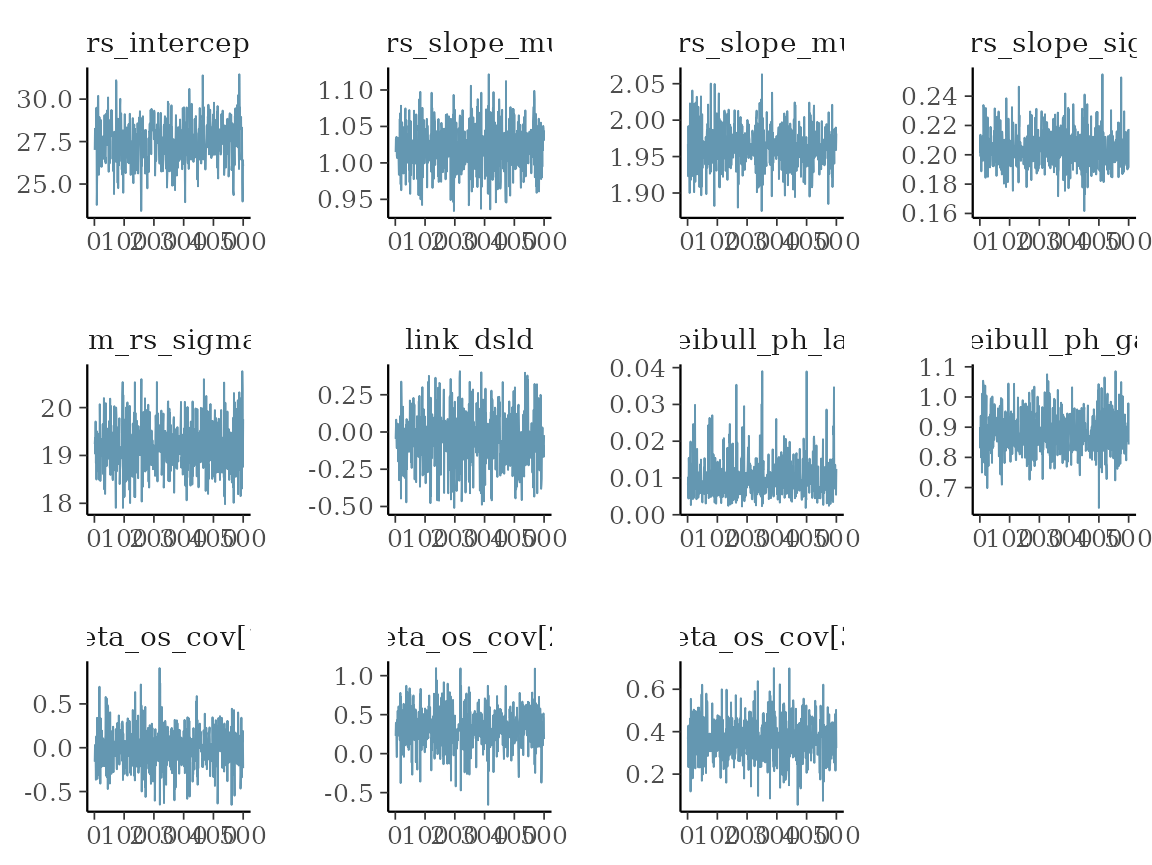

Longitudinal fit plots

Using the longitudinal() method we can extract the longitudinal fit samples from the result, and then plot them for all subjects or those that we are interested in. For illustration, we will plot here the first 10 subjects:

selected_subjects <- head(os_data$subject, 10)
long_quantities <- LongitudinalQuantities(
    mcmc_results,
    grid = GridFixed(
        subjects = selected_subjects
    )
)
as.data.frame(long_quantities) |> head()
#>         group time  values
#> 1 subject_001    0 27.0085
#> 2 subject_001    0 28.2532
#> 3 subject_001    0 27.4511
#> 4 subject_001    0 27.5206
#> 5 subject_001    0 28.1323
#> 6 subject_001    0 29.2868
summary(long_quantities) |> head()
#>         group time   median    lower    upper
#> 1 subject_001    0 27.49175 24.77785 29.76646
#> 2 subject_002    0 27.49175 24.77785 29.76646
#> 3 subject_003    0 27.49175 24.77785 29.76646
#> 4 subject_004    0 27.49175 24.77785 29.76646
#> 5 subject_005    0 27.49175 24.77785 29.76646
#> 6 subject_006    0 27.49175 24.77785 29.76646
autoplot(long_quantities)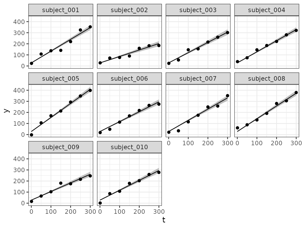

Survival fit plots

And using the SurvivalQuantities() method we can do the same for the estimated survival functions.

surv_quantities <- SurvivalQuantities(
    mcmc_results,
    grid = GridFixed(
        subjects = selected_subjects
    )
)
as.data.frame(surv_quantities) |> head()
#>         group time values
#> 1 subject_001    0      1
#> 2 subject_001    0      1
#> 3 subject_001    0      1
#> 4 subject_001    0      1
#> 5 subject_001    0      1
#> 6 subject_001    0      1
summary(surv_quantities) |> head()
#>         group time median lower upper
#> 1 subject_001    0      1     1     1
#> 2 subject_002    0      1     1     1
#> 3 subject_003    0      1     1     1
#> 4 subject_004    0      1     1     1
#> 5 subject_005    0      1     1     1
#> 6 subject_006    0      1     1     1
autoplot(surv_quantities)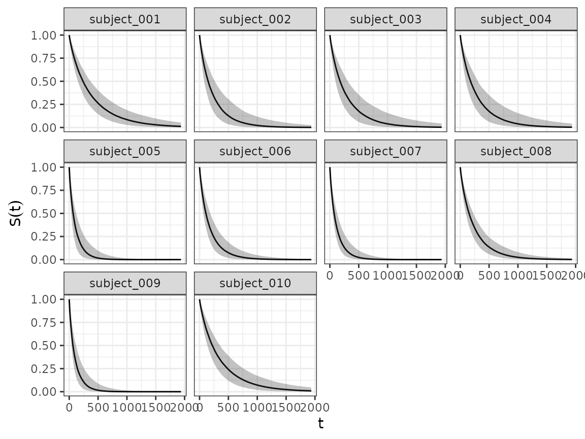

We can also aggregate the estimated survival curves from groups of subjects, using the corresponding method.

surv_quantities <- SurvivalQuantities(
    mcmc_results,
    grid = GridGrouped(
        groups = split(os_data$subject, os_data$arm)
    )
)
autoplot(surv_quantities, add_km = TRUE)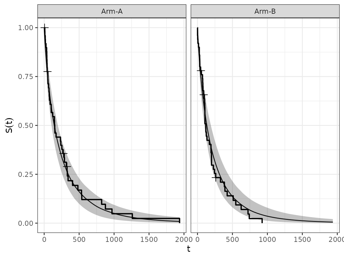

Predicting Survival Quantities for Hypothetical Subjects

The SurvivalQuantities() method can also be used to predict survival quantities for hypothetical subjects with any arbitrary covariate and longitudinal model parameter values. This is done via passing a GridPrediction() object to the method where the newdata and params arguments are used to specify the desired values for the covariates and longitudinal model parameters respectively. For example below we use these functions to predict the survival distribution for a hypothetical subject:

surv_quantities <- SurvivalQuantities(
    mcmc_results,
    grid = GridPrediction(
        times = seq(1, 800, by = 50),
        newdata = dplyr::tibble(
            cov_cat = c("A", "B"),
            cov_cont = c(1.2, 2)
        ),
        params = list(
            intercept = 40,
            slope = 0.05
        )
    )
)
autoplot(surv_quantities)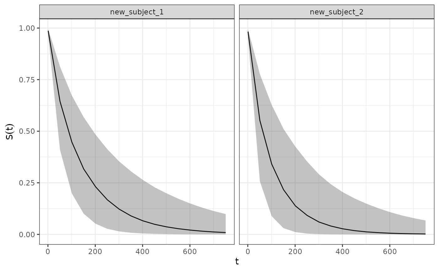

The exact names that are required for the params argument (i.e. the longitudinal model parameters) can be found by running getPredictionNames() on the longitudinal model object. For example:

getPredictionNames(LongitudinalGSF())
#> [1] "b"   "s"   "g"   "phi"

Brier Score

The brierScore() method can be used to extract the Brier Scores (predictive performance measure) from our SurvivalQuantities object.

sq <- SurvivalQuantities(
    mcmc_results,
    grid = GridFixed(times = c(1, 50, 100, 400, 800)),
    type = "surv"
)
brierScore(sq)
#>          1         50        100        400        800 
#> 0.01951765 0.17191088 0.23729063 0.14886106 0.06119522

Initial Values

By default jmpost will set the initial values for all parameters to be a random value drawn from the prior distribution that has been shrunk towards the mean of said distribution e.g. for a prior_normal(4, 2) the initial value for each chain will be:

4 * shrinkage_factor + rnorm(1, 4, 2) * (1 - shrinkage_factor)

Note that the shrinkage factor is set to 0.5 by default and can be changed via the jmpost.prior_shrinkage option e.g.

options("jmpost.prior_shrinkage" = 0.7)

If you wish to manually specify the initial values you can do so via the initialValues() function. For example:

joint_model <- JointModel(
    longitudinal = LongitudinalRandomSlope(),
    survival = SurvivalExponential(),
    link = linkNone()
)
initial_values <- initialValues(joint_model, n_chains = 2)

initial_values[[1]]$lm_rs_intercept <- 0.2
initial_values[[2]]$lm_rs_intercept <- 0.3

mcmc_results <- sampleStanModel(
    joint_model,
    data = DataJoint(...),
    init = initial_values,
    chains = 2
)

Note the following: - initialValues() will return a list of lists where each sublist contains the initial values for the corresponding chain index. - initialValues() by default just returns 1 initial value for each parameter; the sampleStanModel() function will then broadcast this number as many times as required e.g. if you have 3 covariates in your survival model then the initial value for the Beta coeficient will be repeated 3 times. If however you want to specify individual initial values for each covariate you can do so by passing in a vector of the same length as the number of covariates. - initialValues() will not check if the proposed values are valid for constrained parameters. That is, if you are using a prior_cauchy(0, 1) prior for a parameter that should be >0 then you will need to manually set the initial value (as described above) to ensure that it is a valid value. - For constrained parameters (e.g. variance parameters that must be $> 0$ ) initialValues() will continuously sample and discard initial values until it generates one that meet the constraints. If after 100 attempts no valid initial value has been found then it will throw an error.