Analyzing the PRIME Study Data

Introduction

This vignette prepares data from the PRIME study (ClinicalTrials.gov NCT00364013) for analysis with jmpost. PRIME was a randomised, multicentre, phase III study in previously untreated metastatic colorectal cancer. It compared first-line FOLFOX alone with FOLFOX plus panitumumab: 1,183 participants were randomised, with 590 in the comparator arm and 593 in the panitumumab arm. The study’s primary aim was to assess whether adding panitumumab improved progression-free survival (PFS), with overall survival, response, duration of response, time to progression, and safety assessed as secondary outcomes. The study completed in August 2009.

Data

We are fortunate to have access to the PRIME study data via Project Data Sphere (RRID:SCR_003726) (Green et al. 2015). The supplied data are ADaM-format SAS datasets. We begin with the subject-level dataset (adsl) to obtain each participant’s treatment assignment and survival or PFS outcome. Longitudinal tumour measurements are taken from the lesion dataset (adls): VISITDY provides the analysis time and LSSLD is the sum of longest diameters used as the tumour-size marker. We retain the participant identifier (SUBJID) in both datasets so that the subject-level event information can be joined to the repeated measurements. The biomarker (biomark) dataset contains the KRAS mutation status for each participant.

First we read the datasets from the supplied zip file, using a simple helper function:

library(jmpost)
zip_file <- system.file("extdata", "prime_subset.zip", package = "jmpost")

adsl <- read_sas7bdat_from_zip(zip_file, "adsl_pds2019.sas7bdat")
adls <- read_sas7bdat_from_zip(zip_file, "adls_pds2019.sas7bdat")
biomark <- read_sas7bdat_from_zip(zip_file, "biomark_pds2019.sas7bdat")

Next we create the analysis datasets:

kras0 <- biomark |>
  dplyr::select("SUBJID", "BMMTR1")

event_df0 <- adsl |>
  dplyr::left_join(kras0, by = "SUBJID") |>
  dplyr::mutate(STUDY = "1", EVENTYR = DTHDY / 365.25, EVENTFL = DTH) |>
  dplyr::select(
    "SUBJID", "STUDY", "ATRT", "EVENTYR", "EVENTFL",
    "AGE", "SEX",
    ECOG = "B_ECOG", "DIAGTYPE", "LIVERMET",
    KRAS = "BMMTR1"
  ) |>
  dplyr::mutate(
    LIVERMET = factor(LIVERMET, levels = c("N", "Y")),
    KRAS = factor(KRAS, levels = c("Wild-type", "Mutant")),
    PRIMARY_SITE = factor(DIAGTYPE, levels = c("Colon", "Rectal")),
    ECOG_BIN = forcats::fct_collapse(
      dplyr::na_if(as.character(ECOG), ""),
      "0" = "Fully active",
      "1+" = c(
        "In bed less than 50% of the time",
        "Symptoms but ambulatory"
      )
    )
  ) |>
  dplyr::select(
    "SUBJID", "STUDY", "ATRT", "EVENTYR", "EVENTFL",
    "AGE", "SEX", "ECOG_BIN", "KRAS", "LIVERMET", "PRIMARY_SITE"
  )

uid_event0 <- unique(event_df0$SUBJID)

biom_df0 <- adls |>
  dplyr::filter(LSCAT == "Target lesion", !is.na(LSSLD)) |>
  dplyr::mutate(STUDY = "1", BIOMYR = VISITDY / 365.25, BIOMVAL = LSSLD) |>
  dplyr::group_by(SUBJID, VISITDY) |>
  dplyr::slice(1) |>
  dplyr::ungroup() |>
  dplyr::select("SUBJID", "BIOMYR", "BIOMVAL", "VISITDY") |>
  dplyr::filter_out(dplyr::when_any(
    SUBJID == "000424" & VISITDY == 442,
    SUBJID == "000442" & VISITDY == 238,
    SUBJID == "000710"
  ))

baseline_sld <- biom_df0 |>
  dplyr::group_by(SUBJID) |>
  dplyr::filter(VISITDY <= 0) |>
  dplyr::filter(VISITDY == max(VISITDY)) |>
  dplyr::summarize(BASE_SLD = BIOMVAL)

uid_biom0 <- unique(baseline_sld$SUBJID)

retain_uid <- intersect(uid_event0, uid_biom0)
event_df <- event_df0 |>
  na.omit() |>
  dplyr::filter(SUBJID %in% retain_uid) |>
  dplyr::left_join(baseline_sld, by = "SUBJID")

desn0 <- event_df0 |>
  dplyr::filter(SUBJID %in% retain_uid) |>
  dplyr::select(SUBJID, STUDY, ATRT)

biom_df <- biom_df0 |>
  dplyr::filter(SUBJID %in% retain_uid) |>
  dplyr::left_join(desn0, by = "SUBJID")

Because we want to use baseline covariates in the analysis, we need to make sure that we have discarded patients with missing baseline covariates.

So in the end we have two analysis datasets:

• event_df with 428 rows contains the subject-level information including the survival (EVENTYR is the time to event in years, and EVENTFL is the event indicator with 1 indicating the patient died and 0 if the time is censored), and
• biom_df with 2474 rows contains the longitudinal tumour measurements (with BIOMYR as the time in years and BIOMVAL as the sum of longest diameters in millimeters). Here we have filtered out certain observations for subject IDs 000424, 000442, and 000710.

head(event_df)
#> # A tibble: 6 × 12
#>   SUBJID STUDY ATRT          EVENTYR EVENTFL   AGE SEX   ECOG_BIN KRAS  LIVERMET
#>   <chr>  <chr> <chr>           <dbl>   <dbl> <dbl> <chr> <fct>    <fct> <fct>   
#> 1 000003 1     Panitumumab …   0.824       1    65 Male  1+       Muta… Y       
#> 2 000007 1     Panitumumab …   0.928       1    52 Fema… 1+       Muta… Y       
#> 3 000010 1     FOLFOX alone    1.51        1    54 Fema… 0        Muta… Y       
#> 4 000013 1     Panitumumab …   0.539       1    54 Male  0        Wild… Y       
#> 5 000016 1     FOLFOX alone    0.868       1    31 Male  0        Muta… Y       
#> 6 000017 1     FOLFOX alone    2.86        0    57 Fema… 0        Muta… Y       
#> # ℹ 2 more variables: PRIMARY_SITE <fct>, BASE_SLD <dbl>
head(biom_df)
#> # A tibble: 6 × 6
#>   SUBJID   BIOMYR BIOMVAL VISITDY STUDY ATRT                
#>   <chr>     <dbl>   <dbl>   <dbl> <chr> <chr>               
#> 1 000001 -0.0767      426     -28 1     FOLFOX alone        
#> 2 000001 -0.00821     452      -3 1     FOLFOX alone        
#> 3 000001  0.156       464      57 1     FOLFOX alone        
#> 4 000003 -0.0301      118     -11 1     Panitumumab + FOLFOX
#> 5 000003  0.151       110      55 1     Panitumumab + FOLFOX
#> 6 000007 -0.0383      575     -14 1     Panitumumab + FOLFOX

The SUBJID variable serves as the unique identifier for each participant across both datasets.

We also center and scale the two continuous covariates, age and baseline SLD:

event_df <- event_df |>
  dplyr::mutate(AGE = scale(AGE), BASE_SLD = scale(BASE_SLD))

This is important to have the coefficients on the same scale and thus help with the prior setting and then the convergence of the MCMC sampling.

Analysis

Now let’s continue with the joint model analysis using the jmpost package.

We will use these covariates for overall survival as well as the growth and shrinkage means:

cov_form <- ~ ATRT + AGE + SEX + ECOG_BIN + KRAS + LIVERMET + PRIMARY_SITE + BASE_SLD

First we create the DataJoint object that combines the subject-level and longitudinal data, specifying the appropriate formulas for the longitudinal and survival components:

library(jmpost)

jm_dat <- DataJoint(
  subject = DataSubject(
    data = event_df,
    subject = "SUBJID",
    arm = "ATRT",
    study = "STUDY"
  ),
  longitudinal = DataLongitudinal(
    data = biom_df,
    threshold = 3,
    formula = BIOMVAL ~ BIOMYR
  ),
  survival = DataSurvival(
    data = event_df,
    formula = update(cov_form, Surv(EVENTYR, EVENTFL) ~ .)
  )
)
#> Error:
#> ! There are subjects in `longitudinal` that are not present in `subjects`

Normal priors

Next we specify the joint model including the same covariates now for the longitudinal component:

jm_spec <- JointModel(
  longitudinal = LongitudinalSteinFojoCov(
    # Baseline - there is only one study here so just intercept:
    mu_b_formula = ~1,
    omega_b_formula = ~1,
    # Shrinkage - include covariates for the mean:
    mu_s_formula = cov_form,
    omega_s_formula = ~1,
    # Growth - include covariates for the mean:
    mu_g_formula = cov_form,
    omega_g_formula = ~1,
    # Baseline intercept priors:
    mu_b_intercept_prior = prior_normal(4.09434, 1),
    omega_b_intercept_prior = prior_normal(-1.60944, 1),
    # Shrinkage priors:
    mu_s_intercept_prior = prior_normal(-0.69315, 1),
    mu_s_coefficients_prior = prior_normal(0, 1),
    omega_s_intercept_prior = prior_normal(-1.60944, 1),
    # Growth priors:
    mu_g_intercept_prior = prior_normal(-1.20397, 1),
    mu_g_coefficients_prior = prior_normal(0, 1),
    omega_g_intercept_prior = prior_normal(-1.60944, 1),
    sigma = prior_lognormal(log(10), 1)
  ),
  survival = SurvivalWeibullPH(beta = prior_normal(0, 1)),
  # For a 10 mm/year difference, this puts approximately 95% prior probability on hazard ratios between 0.38 and 2.66:
  link = linkDSLD(prior = prior_normal(0, 0.05))
)

Then we can run our MCMC sampler:

We start with a small HMC step size to reduce numerical underflow in early proposals. Stan continues to adapt the step size during warmup. These settings do not establish that 100 warmup iterations are sufficient for the final analysis.

jm_samples_file <- "samples/jm_samples_clean.rds"
if (file.exists(jm_samples_file)) {
  jm_samples <- readRDS(jm_samples_file)
} else {
  options("jmpost.prior_shrinkage" = 0.999)
  set.seed(12345) # Reproduce the initial values generated in R.
  jm_samples <- sampleStanModel(
    jm_spec,
    data = jm_dat,
    iter_warmup = 1000,
    iter_sampling = 1000,
    # smaller starting step eliminated the gamma/lognormal exceptions:
    step_size = 0.001,
    chains = 4,
    parallel_chains = 4,
    seed = 12345
  )
  saveObject(jm_samples, file = jm_samples_file)
}

Let’s check the convergence of the MCMC chains for the population level parameters:

pop_pars <- c(
  "lm_sfc_mu_b_intercept",
  "lm_sfc_mu_g_intercept",
  "lm_sfc_mu_g_coefficients",
  "lm_sfc_mu_s_intercept",
  "lm_sfc_mu_s_coefficients",
  "lm_sfc_omega_b_intercept",
  "lm_sfc_omega_g_intercept",
  "lm_sfc_omega_s_intercept",
  "lm_sfc_sigma",
  "sm_weibull_ph_gamma",
  "sm_weibull_ph_lambda",
  "beta_os_cov",
  "link_coefficients"
)

jm_mcmc <- cmdstanr::as.CmdStanMCMC(jm_samples)
jm_summary <- jm_mcmc$summary(pop_pars)
summary(jm_summary$rhat)
#>    Min. 1st Qu.  Median    Mean 3rd Qu.    Max. 
#>   1.000   1.001   1.002   1.005   1.007   1.024

Here we see that the sampling worked ok, as all the R-hat values are around 1.

This is also confirmed when looking at the trace plots:

jm_draws <- jm_mcmc$draws(pop_pars)

library(bayesplot)
mcmc_trace(jm_draws)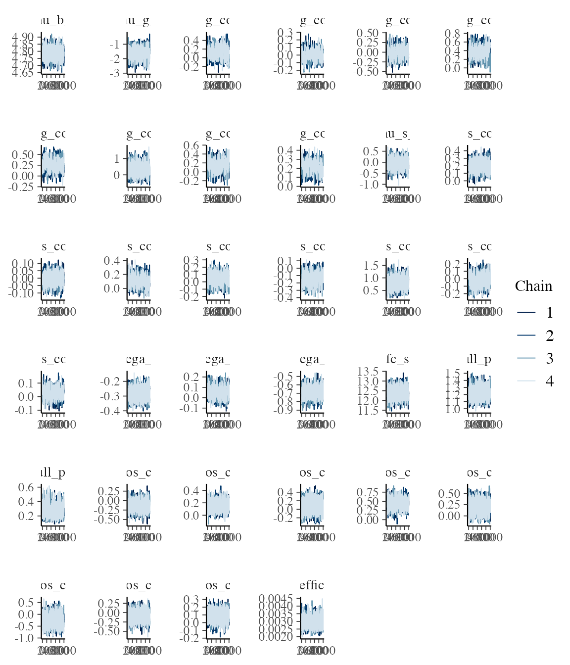

plot of chunk unnamed-chunk-4

We can now inspect the covariate coefficients for overall survival (OS), tumour growth and tumour shrinkage. As in the covariate-selection vignette, coef() uses the fitted design-matrix column names to label the posterior summaries automatically. The growth and shrinkage models use the same covariate formula here. The table reports posterior medians and 90% credible intervals (q5 to q95), alongside R-hat and bulk effective sample size.

coefficient_summary <- coef(jm_samples) |>
  dplyr::mutate(
    component = dplyr::case_when(
      component == "survival" ~ "OS",
      predictor == "mu_g" ~ "Growth",
      predictor == "mu_s" ~ "Shrinkage"
    )
  ) |>
  dplyr::select(component, covariate, median, q5, q95, rhat, ess_bulk)
knitr::kable(coefficient_summary, digits = 3)

component	covariate	median	q5	q95	rhat	ess_bulk
OS	ATRTPanitumumab + FOLFOX	-0.131	-0.347	0.087	1.002	3628.593
OS	AGE	0.156	0.038	0.277	1.001	3857.023
OS	SEXMale	0.077	-0.150	0.302	1.001	3150.267
OS	ECOG_BIN1+	0.448	0.237	0.660	1.002	3408.732
OS	KRASMutant	0.205	-0.008	0.424	1.000	3679.880
OS	LIVERMETY	-0.247	-0.620	0.159	1.001	2622.121
OS	PRIMARY_SITERectal	-0.093	-0.313	0.124	1.001	3709.880
OS	BASE_SLD	0.094	-0.022	0.201	1.002	4909.650
Shrinkage	ATRTPanitumumab + FOLFOX	0.196	0.082	0.315	1.007	859.717
Shrinkage	AGE	-0.010	-0.073	0.052	1.003	854.523
Shrinkage	SEXMale	0.114	-0.005	0.242	1.008	717.072
Shrinkage	ECOG_BIN1+	0.038	-0.087	0.159	1.007	894.919
Shrinkage	KRASMutant	-0.137	-0.267	-0.009	1.004	737.480
Shrinkage	LIVERMETY	0.805	0.478	1.178	1.000	1023.540
Shrinkage	PRIMARY_SITERectal	-0.013	-0.139	0.108	1.007	828.066
Shrinkage	BASE_SLD	0.025	-0.037	0.085	1.012	591.301
Growth	ATRTPanitumumab + FOLFOX	0.122	-0.081	0.340	1.008	445.659
Growth	AGE	0.009	-0.095	0.116	1.017	396.401
Growth	SEXMale	-0.003	-0.237	0.219	1.005	349.918
Growth	ECOG_BIN1+	0.365	0.148	0.579	1.024	340.114
Growth	KRASMutant	0.283	0.059	0.483	1.013	353.553
Growth	LIVERMETY	0.331	-0.173	0.911	1.002	859.491
Growth	PRIMARY_SITERectal	0.141	-0.082	0.361	1.016	372.525
Growth	BASE_SLD	0.217	0.108	0.319	1.014	337.689

The OS coefficients are on the log-hazard scale: exponentiating a coefficient gives the hazard ratio, conditional on the other covariates and the linked tumour trajectory. The growth and shrinkage coefficients act on the log scale of their respective rates, so exponentiating them gives a ratio of the population median rates. Positive coefficients therefore indicate higher mortality hazard, faster growth or faster shrinkage, respectively. For age and baseline SLD, each coefficient describes a one-standard-deviation increase; factor coefficients compare the named level with its reference level. Intervals that span zero indicate uncertainty about the direction of the association.

Horseshoe priors

We can also try to use horseshoe priors in order to do variable selection:

We use partial non-centring for the horseshoe coefficients and centre the subject-specific growth and shrinkage effects. These choices change the sampling coordinates while preserving the prior distributions and likelihood. The scale_noncentred argument below is a computational tuning parameter, separate from the global shrinkage and slab scales. Note that a longer warmup or sampling run alone did not resolve divergent transitions or persistent treedepth saturation.

jm_horseshoe_spec <- JointModel(
  longitudinal = LongitudinalSteinFojoCov(
    # Baseline - there is only one study here so just intercept:
    mu_b_formula = ~1,
    omega_b_formula = ~1,
    # Shrinkage - include covariates for the mean:
    mu_s_formula = cov_form,
    omega_s_formula = ~1,
    # Growth - include covariates for the mean:
    mu_g_formula = cov_form,
    omega_g_formula = ~1,
    # Baseline intercept priors:
    mu_b_intercept_prior = prior_normal(4.09434, 1),
    omega_b_intercept_prior = prior_normal(-1.60944, 1),
    # Shrinkage priors:
    mu_s_intercept_prior = prior_normal(-0.69315, 1),
    mu_s_coefficients_prior = prior_horseshoe(scale_noncentred = 0.1),
    omega_s_intercept_prior = prior_normal(-1.60944, 1),
    # Growth priors:
    mu_g_intercept_prior = prior_normal(-1.20397, 1),
    mu_g_coefficients_prior = prior_horseshoe(scale_noncentred = 0.1),
    omega_g_intercept_prior = prior_normal(-1.60944, 1),
    sigma = prior_lognormal(log(10), 1),
    centred_shrinkage = TRUE,
    centred_growth = TRUE
  ),
  survival = SurvivalWeibullPH(
    beta = prior_horseshoe(scale_noncentred = 0.1)
  ),
  # For a 10 mm/year difference, this puts approximately 95% prior probability on hazard ratios between 0.38 and 2.66:
  link = linkDSLD(prior = prior_normal(0, 0.05))
)

Then we can run our MCMC sampler:

jm_horseshoe_samples_file <- "samples/jm_horseshoe_samples.rds"
if (file.exists(jm_horseshoe_samples_file)) {
  jm_horseshoe_samples <- readRDS(jm_horseshoe_samples_file)
} else {
  options("jmpost.prior_shrinkage" = 0.999)
  set.seed(54321) # Reproduce the initial values generated in R.
  jm_horseshoe_samples <- sampleStanModel(
    jm_horseshoe_spec,
    data = jm_dat,
    iter_warmup = 1000,
    iter_sampling = 1000,
    step_size = 0.001,
    chains = 4,
    parallel_chains = 4,
    seed = 24680
  )
  saveObject(jm_horseshoe_samples, file = jm_horseshoe_samples_file)
}

Let’s check again the convergence:

jm_horseshoe_mcmc <- cmdstanr::as.CmdStanMCMC(jm_horseshoe_samples)
jm_horseshoe_mcmc$diagnostic_summary()
#> $num_divergent
#> [1] 1 0 0 0
#> 
#> $num_max_treedepth
#> [1] 0 0 0 0
#> 
#> $ebfmi
#> [1] 0.5881847 0.5840649 0.5809806 0.5859222

We assess convergence using the sampler diagnostics above. We see that across the 4 chains there was only a single divergent transition, none reached the maximum treedepth and the E-BFMI (Energy Bayesian Fraction of Missing Information) values are above 0.5, where already values above 0.3 would indicate good exploration of the posterior.

Let’s check the traceplots:

jm_horseshoe_draws <- jm_horseshoe_mcmc$draws(pop_pars)
mcmc_trace(jm_horseshoe_draws)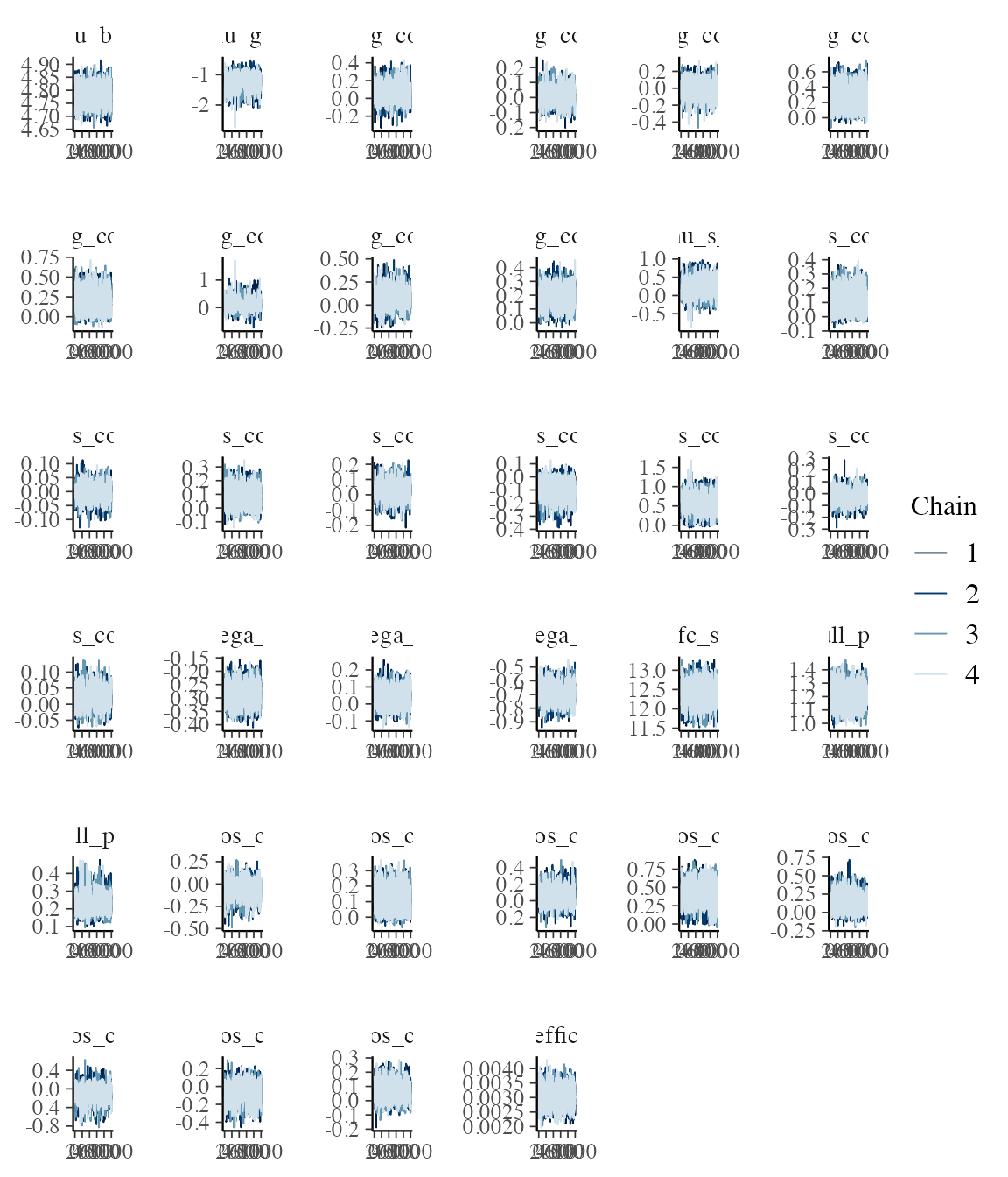

plot of chunk unnamed-chunk-6

These look good, too.

Let’s look at the shrinkage factors:

shrinkage_draws <- shrinkage(jm_horseshoe_samples)
shrinkage_summary <- summary(shrinkage_draws)

Let’s tabulate the variable, median and 5% and 95% quantiles:

shrinkage_summary |>
  dplyr::select(variable, median, q5, q95) |>
  knitr::kable(digits = 3)

variable	median	q5	q95
longitudinal.mu_s:ATRTPanitumumab + FOLFOX	0.996	0.861	1.000
longitudinal.mu_s:AGE	1.000	0.980	1.000
longitudinal.mu_s:SEXMale	0.998	0.925	1.000
longitudinal.mu_s:ECOG_BIN1+	0.999	0.966	1.000
longitudinal.mu_s:KRASMutant	0.998	0.908	1.000
longitudinal.mu_s:LIVERMETY	0.938	0.156	0.997
longitudinal.mu_s:PRIMARY_SITERectal	0.999	0.961	1.000
longitudinal.mu_s:BASE_SLD	1.000	0.970	1.000
longitudinal.mu_g:ATRTPanitumumab + FOLFOX	0.998	0.884	1.000
longitudinal.mu_g:AGE	0.999	0.924	1.000
longitudinal.mu_g:SEXMale	0.999	0.904	1.000
longitudinal.mu_g:ECOG_BIN1+	0.982	0.514	1.000
longitudinal.mu_g:KRASMutant	0.990	0.717	1.000
longitudinal.mu_g:LIVERMETY	0.997	0.771	1.000
longitudinal.mu_g:PRIMARY_SITERectal	0.998	0.872	1.000
longitudinal.mu_g:BASE_SLD	0.989	0.742	0.999
ATRTPanitumumab + FOLFOX	0.998	0.881	1.000
AGE	0.995	0.833	1.000
SEXMale	0.998	0.888	1.000
ECOG_BIN1+	0.962	0.337	0.998
KRASMutant	0.996	0.787	1.000
LIVERMETY	0.998	0.780	1.000
PRIMARY_SITERectal	0.998	0.887	1.000
BASE_SLD	0.998	0.911	1.000

We see here that most covariates have high shrinkage values close to 1, which indicates that the covariate is not so important for the outcome it is used to model. Exceptions where the 95% quantile is below 1 are the following:

• longitudinal.mu_s:LIVERMETY: liver metastases on shrinkage
• longitudinal.mu_g:BASE_SLD: baseline SLD on growth
• ECOG_BIN1+: ECOG 1+/0 on survival hazard

And we can compare that with the coefficient estimates:

coef(jm_horseshoe_samples) |>
  dplyr::mutate(
    component = dplyr::case_when(
      component == "survival" ~ "OS",
      predictor == "mu_g" ~ "Growth",
      predictor == "mu_s" ~ "Shrinkage"
    )
  ) |>
  dplyr::select(component, covariate, median, q5, q95) |>
  knitr::kable(digits = 3)

component	covariate	median	q5	q95
OS	ATRTPanitumumab + FOLFOX	-0.020	-0.218	0.084
OS	AGE	0.119	0.003	0.244
OS	SEXMale	0.015	-0.091	0.210
OS	ECOG_BIN1+	0.431	0.181	0.648
OS	KRASMutant	0.090	-0.034	0.330
OS	LIVERMETY	-0.016	-0.350	0.133
OS	PRIMARY_SITERectal	-0.023	-0.231	0.081
OS	BASE_SLD	0.042	-0.026	0.158
Shrinkage	ATRTPanitumumab + FOLFOX	0.119	-0.002	0.246
Shrinkage	AGE	-0.001	-0.045	0.040
Shrinkage	SEXMale	0.054	-0.018	0.195
Shrinkage	ECOG_BIN1+	0.005	-0.053	0.104
Shrinkage	KRASMutant	-0.075	-0.216	0.010
Shrinkage	LIVERMETY	0.594	0.208	0.962
Shrinkage	PRIMARY_SITERectal	-0.004	-0.098	0.062
Shrinkage	BASE_SLD	0.009	-0.024	0.067
Growth	ATRTPanitumumab + FOLFOX	0.015	-0.077	0.198
Growth	AGE	0.004	-0.065	0.090
Growth	SEXMale	-0.002	-0.154	0.129
Growth	ECOG_BIN1+	0.283	0.021	0.525
Growth	KRASMutant	0.195	-0.005	0.437
Growth	LIVERMETY	0.020	-0.152	0.445
Growth	PRIMARY_SITERectal	0.027	-0.070	0.233
Growth	BASE_SLD	0.192	0.075	0.303

Also here we see that the 95% credible interval excludes 0 for the covariates we have seen with shrinkage factors below 1:

• ECOG_BIN1+ on survival
• LIVERMETY on shrinkage
• BASE_SLD on growth

Interestingly we also see in addition

• AGE on survival
• ECOG_BIN1+ on growth

(Indeed if we use 4 digits for rounding the upper quantile above then we can also see them there already.)

Reproducing NONMEM results

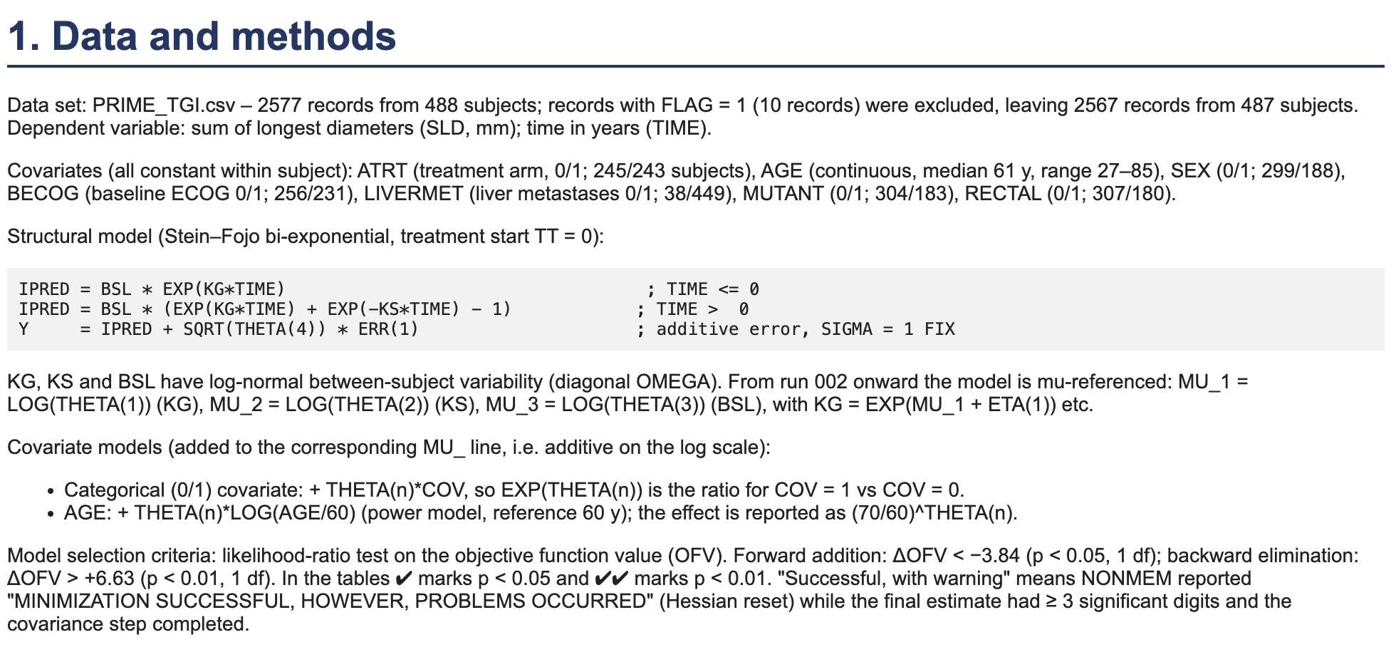
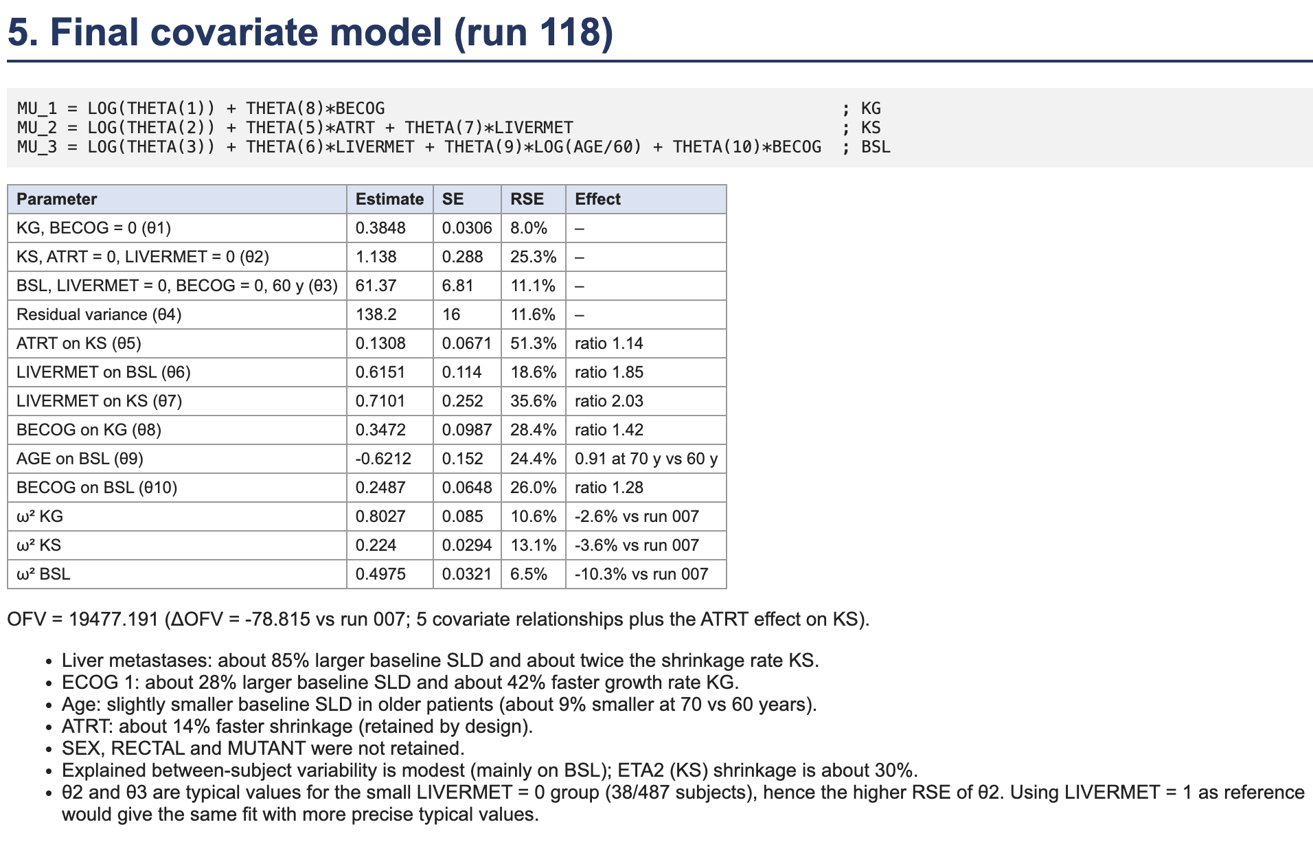
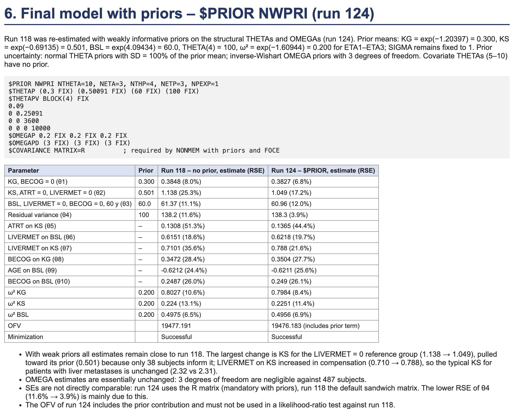
Finally we are going to try to reproduce results from NONMEM on the same data set. We include here some relevant snapshots.

NONMEM Data and methods section

NONMEM Final covariate model results

NONMEM Final parameter estimates

The NONMEM model

The NONMEM model is a longitudinal-only Stein-Fojo tumour growth inhibition (TGI) model, i.e. there is no survival submodel and no link. With time $t$ in years (treatment start at $t = 0$) the sum of longest diameters (SLD) of subject $i$ is

$$y_{ij} = \mathrm{BSL}_i \left(\exp(\mathrm{KG}_i t_{ij}) + \exp(-\mathrm{KS}_i t_{ij}) - 1\right) + \varepsilon_{ij} \quad (t_{ij} > 0), \qquad y_{ij} = \mathrm{BSL}_i \exp(\mathrm{KG}_i t_{ij}) + \varepsilon_{ij} \quad (t_{ij} \leq 0),$$

with additive normal residual error $\varepsilon_{ij} \sim N(0, \theta_4)$, where $\theta_4$ is a variance. This is the same structural model as LongitudinalSteinFojoCov. The growth rate KG, the shrinkage rate KS and the baseline BSL are log-normally distributed with independent random effects (diagonal $\Omega$). The final covariate model (run 118, also used in run 124) is explicitly

$$\begin{aligned} \mathrm{KG}_i &= \theta_1 \exp\left(\theta_8\,\mathrm{BECOG}_i + \eta_{1i}\right), \\ \mathrm{KS}_i &= \theta_2 \exp\left(\theta_5\,\mathrm{ATRT}_i + \theta_7\,\mathrm{LIVERMET}_i + \eta_{2i}\right), \\ \mathrm{BSL}_i &= \theta_3 \left(\frac{\mathrm{AGE}_i}{60}\right)^{\theta_9} \exp\left(\theta_6\,\mathrm{LIVERMET}_i + \theta_{10}\,\mathrm{BECOG}_i + \eta_{3i}\right), \\ \eta_i &\sim N_3\!\left(0, \operatorname{diag}(\omega^2_{KG},\omega^2_{KS},\omega^2_{BSL})\right). \end{aligned}$$

Here BECOG is 0 for ECOG 0 and 1 for ECOG 1+, ATRT is 0 for FOLFOX alone and 1 for panitumumab + FOLFOX, and LIVERMET is 0 for no and 1 for yes. The typical values $\theta_1$, $\theta_2$ and $\theta_3$ are conditional population medians. The covariate relationships are summarised below:

Parameter	Covariates (effect on the log scale)
KG (growth)	BECOG (ECOG 1+ vs 0)
KS (shrinkage)	ATRT (panitumumab + FOLFOX vs FOLFOX alone), LIVERMET (liver metastases yes vs no)
BSL (baseline)	LIVERMET, BECOG, and age as log(AGE / 60) (power model, reference age 60 years)

Note that the continuous covariate (age) is therefore not centred and scaled as above, and that the reference group for the typical values $\theta_1$ to $\theta_3$ is: ECOG 0, no liver metastases, FOLFOX alone (for KS only), age 60. SEX, RECTAL (primary site) and MUTANT (KRAS) were not retained in the NONMEM covariate search.

Run 124 adds the following priors, with all other parameters (the covariate coefficients $\theta_5, \ldots, \theta_{10}$) having no prior, i.e. flat:

• Typical values on the natural (not log) scale, independent normal priors with standard deviation equal to the prior mean: $\theta_1$ (KG) $\sim N(0.3, 0.3^2)$, $\theta_2$ (KS) $\sim N(0.50091, 0.50091^2)$, $\theta_3$ (BSL) $\sim N(60, 60^2)$.
• The residual variance $\theta_4 \sim N(100, 100^2)$.
• The three random effect variances $\omega^2_{KG}, \omega^2_{KS}, \omega^2_{BSL}$ have independent inverse-Wishart priors with prior value $0.2$ and 3 degrees of freedom, which for $1 \times 1$ blocks are inverse-gamma priors with shape $\alpha = \nu / 2 = 1.5$ and scale $\beta = \nu R / 2 = 0.3$. (This is confirmed by the “PRIOR CONSTANT TO OBJECTIVE FUNCTION” of 31.07 in the NONMEM output, which is reproduced exactly by these normal and inverse-gamma densities.)

The control file constrains $\theta_1,\ldots,\theta_4$ to be positive. NONMEM evaluates the normal prior penalties within these bounds; the corresponding Bayesian priors are normal distributions restricted to positive values. Their truncation normalisers are constant because the prior hyperparameters are fixed, so they do not affect the estimates.

Important differences to keep in mind when comparing:

• NONMEM (FOCE-I with priors) reports a penalised maximum likelihood / posterior mode estimate in the parametrisation of $\theta$ and $\Omega$, while jmpost reports posterior summaries (here medians) from a full Bayesian analysis that samples the random effects and marginalises them in the population summaries. FOCE approximates the marginal likelihood, so even matching priors and data do not imply identical estimates. Prior influence can still matter for the reference-group KS, which is informed by only 38 subjects without liver metastases.
• The jmpost parameters are the log typical values, the log standard deviations $\omega$ and the residual standard deviation $\sigma$, whereas the NONMEM priors are on $\theta$, $\omega^2$ and $\theta_4 = \sigma^2$. To reproduce them exactly, priors on these transformed scales (with Jacobian) are needed; see below.

Comparing population posterior modes on the NONMEM scales would remove the mode-versus-median difference, but simply calling CmdStanR’s $optimize() on the current hierarchical Stan model optimises population parameters and patient random effects together. This joint mode is not the population mode after integrating out the random effects, which is the quantity approximated by FOCE with priors. Modes also depend on the parameter scale and Jacobian adjustments. A closer optimisation-based comparison would therefore require an objective that marginalises the random effects and expresses the population density on the NONMEM scales; switching from sampling to optimisation alone does not guarantee closer agreement.

NONMEM estimates

We store the run 124 estimates from NONMEM/PRIME_TGI_124.ext (final-estimate row -1000000000), with relative standard errors from the NONMEM covariance step with the R matrix, and convert them to the jmpost scale for later comparison. These values are embedded here so that rendering does not depend on the original NONMEM output directory:

nonmem_124 <- tibble::tribble(
  ~nonmem, ~predictor, ~covariate, ~estimate, ~rse_percent, ~scale,
  "theta1: KG, ECOG 0", "mu_g", "(Intercept)", 0.382695, 6.8, "log",
  "theta2: KS, FOLFOX alone, no liver metastases", "mu_s", "(Intercept)", 1.04936, 17.2, "log",
  "theta3: BSL, no liver metastases, ECOG 0, age 60", "mu_b", "(Intercept)", 60.9599, 12.0, "log",
  "theta4: residual variance", "sigma", NA, 138.252, 3.9, "sqrt",
  "theta5: ATRT on KS", "mu_s", "ATRTPanitumumab + FOLFOX", 0.136518, 44.4, "identity",
  "theta6: LIVERMET on BSL", "mu_b", "LIVERMETY", 0.621805, 19.7, "identity",
  "theta7: LIVERMET on KS", "mu_s", "LIVERMETY", 0.787987, 21.6, "identity",
  "theta8: BECOG on KG", "mu_g", "ECOG_BIN1+", 0.350402, 27.7, "identity",
  "theta9: AGE on BSL (power, per log(AGE / 60))", "mu_b", "LOG_AGE60", -0.621084, 25.6, "identity",
  "theta10: BECOG on BSL", "mu_b", "ECOG_BIN1+", 0.248961, 26.1, "identity",
  "omega2 KG", "omega_g", "(Intercept)", 0.798437, 8.4, "half_log",
  "omega2 KS", "omega_s", "(Intercept)", 0.225085, 11.4, "half_log",
  "omega2 BSL", "omega_b", "(Intercept)", 0.495594, 6.9, "half_log"
) |>
  dplyr::rowwise() |>
  dplyr::mutate(
    jmpost = switch(scale,
      log = log(estimate),
      sqrt = sqrt(estimate),
      half_log = log(sqrt(estimate)),
      identity = estimate
    )
  ) |>
  dplyr::ungroup()
knitr::kable(nonmem_124, digits = 4)

nonmem	predictor	covariate	estimate	rse_percent	scale	jmpost
theta1: KG, ECOG 0	mu_g	(Intercept)	0.3827	6.8	log	-0.9605
theta2: KS, FOLFOX alone, no liver metastases	mu_s	(Intercept)	1.0494	17.2	log	0.0482
theta3: BSL, no liver metastases, ECOG 0, age 60	mu_b	(Intercept)	60.9599	12.0	log	4.1102
theta4: residual variance	sigma	NA	138.2520	3.9	sqrt	11.7581
theta5: ATRT on KS	mu_s	ATRTPanitumumab + FOLFOX	0.1365	44.4	identity	0.1365
theta6: LIVERMET on BSL	mu_b	LIVERMETY	0.6218	19.7	identity	0.6218
theta7: LIVERMET on KS	mu_s	LIVERMETY	0.7880	21.6	identity	0.7880
theta8: BECOG on KG	mu_g	ECOG_BIN1+	0.3504	27.7	identity	0.3504
theta9: AGE on BSL (power, per log(AGE / 60))	mu_b	LOG_AGE60	-0.6211	25.6	identity	-0.6211
theta10: BECOG on BSL	mu_b	ECOG_BIN1+	0.2490	26.1	identity	0.2490
omega2 KG	omega_g	(Intercept)	0.7984	8.4	half_log	-0.1125
omega2 KS	omega_s	(Intercept)	0.2251	11.4	half_log	-0.7456
omega2 BSL	omega_b	(Intercept)	0.4956	6.9	half_log	-0.3510

Here jmpost is the NONMEM estimate on the scale of the corresponding jmpost parameter: log typical values for the intercepts (lm_sfc_mu_*_intercept), the residual standard deviation (lm_sfc_sigma), the log of the random effect standard deviations (lm_sfc_omega_*_intercept), and unchanged covariate coefficients (lm_sfc_mu_*_coefficients). The OFV of run 124 is 19476.183 (including the prior term); it is not comparable to the jmpost log likelihood.

Data

The NONMEM data set has 487 subjects with 2567 tumour measurements (after removal of 10 flagged records). Since there is no survival part, we do not need the KRAS, sex, primary site and baseline SLD covariates used above, and thus we do not have to drop the subjects with missing values in these. We therefore rebuild the subject-level data with only the covariates that are needed, and we use the raw age (before centring and scaling) to create log(AGE / 60). This second preparation differs from the joint-analysis preparation above: following the reference R script, blank ECOG is assigned BECOG = 0 rather than discarded. This retains subject 000930 and their three measurements. The assignment reproduces the reference analysis’s imputation decision; it does not establish that the subject’s observed ECOG was 0. The tumour measurements and flagged-record exclusions are shared with biom_df0 above.

nm_subject_df <- event_df0 |>
  dplyr::mutate(
    LOG_AGE60 = log(AGE / 60),
    ECOG_BIN = forcats::fct_na_value_to_level(ECOG_BIN, level = "0"),
    SEX = forcats::fct_relevel(SEX, "Male"),
    KRAS = forcats::fct_na_value_to_level(KRAS, level = "Wild-type")
  ) |>
  dplyr::select("SUBJID", "STUDY", "ATRT", "LOG_AGE60", "SEX", "ECOG_BIN", "LIVERMET", "KRAS", "PRIMARY_SITE") |>
  dplyr::filter(SUBJID %in% biom_df0$SUBJID)

nm_biom_df <- biom_df0 |>
  dplyr::filter(SUBJID %in% nm_subject_df$SUBJID) |>
  dplyr::left_join(nm_subject_df[, c("SUBJID", "STUDY", "ATRT")], by = "SUBJID")

# Check that we are using the same data as NONMEM:
stopifnot(
  nrow(nm_subject_df) == 487,
  nrow(nm_biom_df) == 2567
)

We can compare the factor level observation counts with the ones from the NONMEM report to ensure that we (very likely) use the same dataset: “ATRT (treatment arm, 0/1; 245/243 subjects), AGE (continuous, median 61 y, range 27–85), SEX (0/1; 299/188), BECOG (baseline ECOG 0/1; 256/231), LIVERMET (liver metastases 0/1; 38/449), MUTANT (0/1; 304/183), RECTAL (0/1; 307/180).”

table(nm_subject_df$ATRT) # not clear how NONMEM has 243 for Panitumumab + FOLFOX
#> 
#>         FOLFOX alone Panitumumab + FOLFOX 
#>                  245                  242
table(nm_subject_df$ECOG_BIN)
#> 
#>   0  1+ 
#> 256 231
table(nm_subject_df$LIVERMET)
#> 
#>   N   Y 
#>  38 449
table(nm_subject_df$SEX)
#> 
#>   Male Female 
#>    299    188
table(nm_subject_df$KRAS)
#> 
#> Wild-type    Mutant 
#>       304       183
table(nm_subject_df$PRIMARY_SITE)
#> 
#>  Colon Rectal 
#>    307    180

Now that looks ok, and we specify the data object just with subject and longitudinal data:

nm_dat <- DataJoint(
  subject = DataSubject(
    data = nm_subject_df,
    subject = "SUBJID",
    arm = "ATRT",
    study = "STUDY"
  ),
  longitudinal = DataLongitudinal(
    data = nm_biom_df,
    formula = BIOMVAL ~ BIOMYR
  )
)

Note that we do not specify a threshold, so no observations are treated as censored, as in NONMEM.

The jmpost model

The model maps to LongitudinalSteinFojoCov as follows. The mu_* predictors use the default "linear" parametrisation, mu = intercept + X beta, which enters as psi = exp(mu + eta * omega). This is the mu-referenced NONMEM model, e.g. MU_1 = LOG(THETA(1)) + THETA(8) * BECOG: the intercepts are $\log \theta_1, \log \theta_2, \log \theta_3$ and the coefficients are $\theta_5, \ldots, \theta_{10}$. The omega_* predictors use the default "log-linear" parametrisation (intercept-only formulas), so $\omega = \exp(\text{intercept})$. Observation error is additive (scaled_variance = FALSE) with standard deviation sigma $= \sqrt{\theta_4}$.

To reproduce the NONMEM priors, place the distributions on the NONMEM scales using transform. The transformation maps a declared jmpost parameter to the scale on which the density is evaluated; jmpost adds the Jacobian automatically:

1. For mu_{b,s,g}_intercept_prior, use prior_normal(mean, sd, transform = prior_transform_exp()). This places the normal prior on $\theta = \exp(\text{intercept})$, restricted to positive values.
2. For omega_{b,s,g}_intercept_prior, use prior_invgamma(1.5, 0.3, transform = prior_transform_exp(scale = 2)). The density is on $\omega^2 = \exp(2 \cdot \text{intercept})$.
3. For the residual standard deviation sigma, use prior_normal(100, 100, transform = prior_transform_square()). The density is on $\sigma^2$. LongitudinalSteinFojoCov() applies a very small positive lower bound to sigma; the corresponding truncation bound on the density scale is its square.
4. For the covariate coefficients $\theta_5, \ldots, \theta_{10}$, use prior_flat(). This adds no prior density term on the coefficient scale; its default normal distribution is used only for initial values.

These transformations specify prior scales independently of the predictor parametrizations above. The truncation normalisers and the log(2) terms are constant here, so they do not change posterior shape.

We use the default (non-centred) subject-level parametrisation for growth and shrinkage and the centred one for the baseline.

nm_spec <- JointModel(
  longitudinal = LongitudinalSteinFojoCov(
    mu_b_formula = ~ LIVERMET + LOG_AGE60 + ECOG_BIN,
    omega_b_formula = ~1,
    mu_s_formula = ~ ATRT + LIVERMET,
    omega_s_formula = ~1,
    mu_g_formula = ~ECOG_BIN,
    omega_g_formula = ~1,
    mu_b_parametrization = "linear",
    mu_s_parametrization = "linear",
    mu_g_parametrization = "linear",
    omega_b_parametrization = "log-linear",
    omega_s_parametrization = "log-linear",
    omega_g_parametrization = "log-linear",
    # Baseline: theta3 ~ N(60, 60^2) on the positive natural scale.
    mu_b_intercept_prior = prior_normal(
      60, 60,
      transform = prior_transform_exp()
    ),
    mu_b_coefficients_prior = prior_flat(),
    omega_b_intercept_prior = prior_invgamma(
      1.5, 0.3,
      transform = prior_transform_exp(scale = 2)
    ),
    # Shrinkage: theta2 ~ N(0.50091, 0.50091^2).
    mu_s_intercept_prior = prior_normal(
      0.50091, 0.50091,
      transform = prior_transform_exp()
    ),
    mu_s_coefficients_prior = prior_flat(),
    omega_s_intercept_prior = prior_invgamma(
      1.5, 0.3,
      transform = prior_transform_exp(scale = 2)
    ),
    # Growth: theta1 ~ N(0.3, 0.3^2).
    mu_g_intercept_prior = prior_normal(
      0.3, 0.3,
      transform = prior_transform_exp()
    ),
    mu_g_coefficients_prior = prior_flat(),
    omega_g_intercept_prior = prior_invgamma(
      1.5, 0.3,
      transform = prior_transform_exp(scale = 2)
    ),
    # sigma^2 = theta4 ~ N(100, 100^2).
    sigma = prior_normal(
      100, 100,
      transform = prior_transform_square()
    ),
    scaled_variance = FALSE
  )
)

Then we run the sampler:

nm_samples_file <- "samples/nm_samples.rds"
if (file.exists(nm_samples_file)) {
  nm_samples <- readRDS(nm_samples_file)
} else {
  options("jmpost.prior_shrinkage" = 0.999)
  set.seed(2468)
  nm_samples <- sampleStanModel(
    nm_spec,
    data = nm_dat,
    iter_warmup = 1000,
    iter_sampling = 1000,
    chains = 4,
    parallel_chains = 4,
    step_size = 0.001,
    seed = 2468
  )
  saveObject(nm_samples, file = nm_samples_file)
}

Comparison

The saved fit contains four chains with 1,000 post-warmup draws each. We first check the sampler diagnostics and retain the parameter names alongside the summaries on the internal jmpost scales.

nm_pop_pars <- c(
  "lm_sfc_mu_b_intercept",
  "lm_sfc_mu_s_intercept",
  "lm_sfc_mu_g_intercept",
  "lm_sfc_omega_b_intercept",
  "lm_sfc_omega_s_intercept",
  "lm_sfc_omega_g_intercept",
  "lm_sfc_sigma"
)
nm_mcmc <- cmdstanr::as.CmdStanMCMC(nm_samples)
nm_mcmc$diagnostic_summary()
#> $num_divergent
#> [1] 0 0 0 0
#> 
#> $num_max_treedepth
#> [1] 0 0 0 0
#> 
#> $ebfmi
#> [1] 0.5935062 0.6052086 0.5398737 0.5635327
nm_summary <- nm_mcmc$summary(nm_pop_pars)
nm_coef <- coef(nm_samples)

nm_diagnostics <- dplyr::bind_rows(nm_summary, nm_coef) |>
  dplyr::select(variable, median, q5, q95, rhat, ess_bulk)
knitr::kable(nm_diagnostics, digits = 3)

variable	median	q5	q95	rhat	ess_bulk
lm_sfc_mu_b_intercept	4.118	3.908	4.325	1.001	4873.358
lm_sfc_mu_s_intercept	0.020	-0.280	0.290	1.000	1542.152
lm_sfc_mu_g_intercept	-1.077	-1.208	-0.951	1.007	249.676
lm_sfc_omega_b_intercept	-0.335	-0.390	-0.278	1.001	6376.284
lm_sfc_omega_s_intercept	-0.646	-0.743	-0.544	1.003	1038.723
lm_sfc_omega_g_intercept	-0.050	-0.124	0.025	1.002	621.644
lm_sfc_sigma	11.826	11.453	12.239	1.003	1833.788
lm_sfc_mu_b_coefficients[1]	0.607	0.400	0.825	1.003	5280.720
lm_sfc_mu_b_coefficients[2]	-0.626	-0.887	-0.356	1.002	9957.419
lm_sfc_mu_b_coefficients[3]	0.250	0.140	0.364	1.000	9010.584
lm_sfc_mu_s_coefficients[1]	0.138	0.028	0.249	1.006	803.572
lm_sfc_mu_s_coefficients[2]	0.771	0.508	1.066	1.001	1661.253
lm_sfc_mu_g_coefficients[1]	0.350	0.173	0.524	1.011	318.822

There are no divergent transitions or maximum-treedepth hits, and E-BFMI is above 0.5 in every chain. Mixing is slower for the growth intercept and its ECOG coefficient (bulk effective sample sizes approximately 250 and 319; R-hat approximately 1.007 and 1.011). These parameters would benefit from more effective draws before drawing conclusions about small differences.

The same estimands side by side

The next table puts all 13 population parameters on the NONMEM scales: typical KG and KS in inverse years, typical BSL in mm, residual variance in mm squared, covariate coefficients on their original log-effect/power scales, and between-subject variances of the log parameters. Reference groups are those specified above. The jmpost columns are posterior medians and 90% equal-tailed credible intervals, computed after transforming each draw. NONMEM reports FOCE-I estimates with priors and relative standard errors (RSE, %); these RSEs are covariance-step uncertainty measures, not posterior credible intervals.

# Match by predictor and fitted design-matrix names, rather than row order.
nm_parameter_map <- dplyr::bind_rows(
  tibble::tibble(
    predictor = c(
      "mu_b", "mu_s", "mu_g", "omega_b", "omega_s", "omega_g",
      "sigma"
    ),
    covariate = c(rep("(Intercept)", 6), NA_character_),
    variable = nm_pop_pars
  ),
  dplyr::select(nm_coef, predictor, covariate, variable)
)
nm_comparison <- nonmem_124 |>
  dplyr::left_join(
    nm_parameter_map,
    by = c("predictor", "covariate")
  )
stopifnot(
  nrow(nm_comparison) == 13L,
  !anyNA(nm_comparison$variable),
  !anyDuplicated(nm_comparison$variable)
)

nm_comparison_draws <- posterior::as_draws_matrix(
  nm_mcmc$draws(nm_comparison$variable)
)
nm_native_summary <- lapply(seq_len(nrow(nm_comparison)), function(i) {
  draws <- nm_comparison_draws[, nm_comparison$variable[i]]
  # Invert the NONMEM-to-jmpost transformations defined earlier.
  draws <- switch(nm_comparison$scale[i],
    log = exp(draws),
    sqrt = draws^2,
    half_log = exp(2 * draws),
    identity = draws
  )
  tibble::tibble(
    median = median(draws),
    q5 = unname(quantile(draws, 0.05)),
    q95 = unname(quantile(draws, 0.95))
  )
}) |>
  dplyr::bind_rows()
nm_comparison <- dplyr::bind_cols(nm_comparison, nm_native_summary)

nm_comparison |>
  dplyr::transmute(
    Estimand = nonmem,
    `jmpost median` = median,
    `jmpost 5%` = q5,
    `jmpost 95%` = q95,
    `NONMEM estimate` = estimate,
    `NONMEM RSE (%)` = rse_percent
  ) |>
  knitr::kable(digits = 3)

Estimand	jmpost median	jmpost 5%	jmpost 95%	NONMEM estimate	NONMEM RSE (%)
theta1: KG, ECOG 0	0.341	0.299	0.386	0.383	6.8
theta2: KS, FOLFOX alone, no liver metastases	1.020	0.756	1.336	1.049	17.2
theta3: BSL, no liver metastases, ECOG 0, age 60	61.423	49.793	75.536	60.960	12.0
theta4: residual variance	139.847	131.169	149.795	138.252	3.9
theta5: ATRT on KS	0.138	0.028	0.249	0.137	44.4
theta6: LIVERMET on BSL	0.607	0.400	0.825	0.622	19.7
theta7: LIVERMET on KS	0.771	0.508	1.066	0.788	21.6
theta8: BECOG on KG	0.350	0.173	0.524	0.350	27.7
theta9: AGE on BSL (power, per log(AGE / 60))	-0.626	-0.887	-0.356	-0.621	25.6
theta10: BECOG on BSL	0.250	0.140	0.364	0.249	26.1
omega2 KG	0.905	0.781	1.050	0.798	8.4
omega2 KS	0.275	0.226	0.337	0.225	11.4
omega2 BSL	0.512	0.458	0.574	0.496	6.9

The typical growth rate is approximately 0.341/year in jmpost versus 0.383/year in NONMEM; typical shrinkage is 1.020/year versus 1.049/year. Baseline size is approximately 61.4 mm versus 61.0 mm. The covariate effects are close across the two methods, including the treatment effect on shrinkage (approximately 0.138 versus 0.137 on the log scale).

The largest relative differences are in the between-subject variances for log KG and log KS: approximately 0.905 versus 0.798, and 0.275 versus 0.225, respectively. The NONMEM variance estimate for log KS (0.225) lies just below the jmpost 90% credible interval (0.226 to 0.337); the other 12 NONMEM point estimates fall within the corresponding intervals. This is descriptive agreement; the intervals are not a formal test of equivalence. Matching the data, model and priors still leaves the FOCE approximation and posterior-mode versus posterior-median distinction discussed above.

Next steps

First, in order to get closer alignment between the longitudinal model results we could use METHOD = NUTS in the NONMEM software, in order to also run a no-u turn sampler, i.e. Bayesian MCMC.

Second, current NONMEM analysis is a two-stage approach: the tumour growth inhibition (TGI) model above is fitted first, and the overall survival (OS) model is then fitted separately in R (a Weibull survreg model using the individual NONMEM estimates, e.g. log(KG) and baseline SLD, as covariates).

A natural next step is to use a full joint model instead also in NONMEM and get agreement with the jmpost results.

References

Green, Allen K., Stephanie C. Reeder-Hayes, Robert W. Corty, et al. 2015. ‘The Project Data Sphere Initiative: Accelerating Cancer Research by Sharing Data’. The Oncologist 20 (5): 464–70. https://doi.org/10.1634/theoncologist.2014-0431.