Plot comparison of component functions

Usage

g_comparison(
  sculptures,
  descriptions,
  rug_sides = "b",
  missings_spec = missings_specification(),
  facet_spec = facet_specification(),
  hue_coloring = FALSE,
  logodds_to_prob = FALSE
)

Arguments

sculptures: List of objects of classes sculpture.
descriptions: Character vector with model names. Same length as sculptures.
rug_sides: "" for none, "b", for bottom, "trbl" for all 4 sides (see geom_rug)
missings_spec: Object of class missings_specificatoin.
facet_spec: Object of class facet_specificatoin.
hue_coloring: Logical, use hue-based coloring? Defaults to FALSE, meaning that predefined colors will be used instead.
logodds_to_prob: (logical) Only valid for binary response and sculptures built on the log-odds scale. Defaults to FALSE (i.e. no effect). If TRUE, then the y-values are transformed through inverse logit function 1 / (1 + exp(-x)).

Value

List of ggplots (one for continuous features, one for discrete).

Details

The first element of sculptures works as a reference sculpture. All other sculptures must have a subset of variables with respect to the first one (i.e. the same variables or less, but not new ones). This allows to visualize polished together with non-polished sculptures, if the non-polished one is specified as the first one.

Examples

df <- mtcars
df$vs <- as.factor(df$vs)
model <- rpart::rpart(
  hp ~ mpg + carb + vs,
  data = df,
  control = rpart::rpart.control(minsplit = 10)
)
model_predict <- function(x) predict(model, newdata = x)
covariates <- c("mpg", "carb", "vs")
pm <- sample_marginals(df[covariates], n = 50, seed = 5)

rs <- sculpt_rough(
  dat = pm,
  model_predict_fun = model_predict,
  n_ice = 10,
  seed = 1,
  verbose = 0
)

ds <- sculpt_detailed_gam(rs)

# this keeps only "mpg"
ps <- sculpt_polished(ds, k = 1)

# also define simple labels
labels <- structure(
  toupper(covariates), # labels
  names = covariates # current (old) names
)

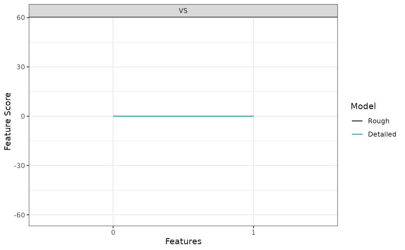
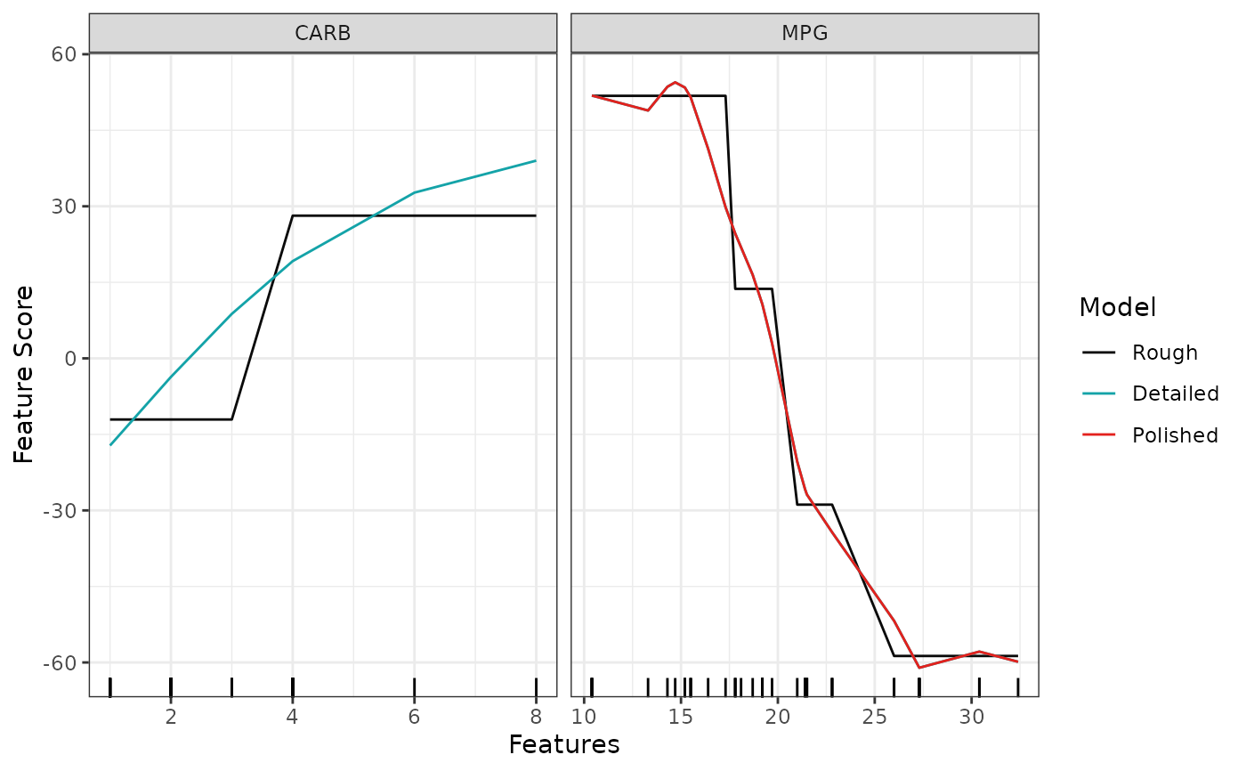
# Component functions of "Detailed" and "Polished" are the same for "mpg" variable,
# therefore red curve overlays the blue one for "mpg"
comp <- g_comparison(
  sculptures = list(rs, ds, ps),
  descriptions = c("Rough", "Detailed", "Polished"),
  facet_spec = facet_specification(ncol = 2, labels = labels)
)
comp$continuous

comp$discrete