Introduction to Model Sculpting • modsculpt

Introduction

The goal of this vignette is to make you familiar with model sculpting. We do this by using a publicly available “bike sharing” dataset.

library(modsculpt)

Data preparation

Download the dataset at http://archive.ics.uci.edu/ml/datasets/Bike+Sharing+Dataset, unzip, and load day.csv. You can use the following code to do all the steps above:

download.file(
  "http://archive.ics.uci.edu/ml/machine-learning-databases/00275/Bike-Sharing-Dataset.zip",
  destfile = "bike_rentals.zip"
)
unzip("bike_rentals.zip")
df <- read.csv("day.csv")

Firstly, check the dimensionality:

dim(df)
#> [1] 731  16

Have a look at the dataset

head(df)
#>   instant     dteday season yr mnth holiday weekday workingday weathersit
#> 1       1 2011-01-01      1  0    1       0       6          0          2
#> 2       2 2011-01-02      1  0    1       0       0          0          2
#> 3       3 2011-01-03      1  0    1       0       1          1          1
#> 4       4 2011-01-04      1  0    1       0       2          1          1
#> 5       5 2011-01-05      1  0    1       0       3          1          1
#> 6       6 2011-01-06      1  0    1       0       4          1          1
#>       temp    atemp      hum windspeed casual registered  cnt
#> 1 0.344167 0.363625 0.805833 0.1604460    331        654  985
#> 2 0.363478 0.353739 0.696087 0.2485390    131        670  801
#> 3 0.196364 0.189405 0.437273 0.2483090    120       1229 1349
#> 4 0.200000 0.212122 0.590435 0.1602960    108       1454 1562
#> 5 0.226957 0.229270 0.436957 0.1869000     82       1518 1600
#> 6 0.204348 0.233209 0.518261 0.0895652     88       1518 1606

In this dataset, instant is the primary key, cnt is the response that we want to predict, columns season:windspeed are the features we can use for prediction.

response <- "cnt"
covariates <- c("season", "yr", "mnth", "holiday", "weekday", "workingday", "weathersit", "temp", "atemp", "hum", "windspeed")

Let’s get rid of instant, dteday, casual and registered:

df$instant <- NULL
df$dteday <- NULL
df$casual <- NULL
df$registered <- NULL

Lastly, we need to properly encode discrete variables into factors:

idx_factor <- vapply(df, function(x) length(unique(x)) <= 12, logical(1))
df[idx_factor] <- lapply(df[idx_factor], as.factor)

We treat the following variables as factors:

print(names(idx_factor)[idx_factor])
#> [1] "season"     "yr"         "mnth"       "holiday"    "weekday"   
#> [6] "workingday" "weathersit"

The goal of this document is to show how model sculpting can be used. Therefore, we will not explore the bike rentals dataset further but rather go ahead with the model sculpting.

Model Sculpting

Build a base model

Before we can move to model sculpting, we need an actual model that we can sculpt. Let’s build an xgboost model. Yet before we start, it is good to check the following:

Investigate the NAs. Check if there are any NAs with the following code:

anyNA(df)
#> [1] FALSE

For model sculpting, you should remove or impute NAs if you have any.

Remove constant (or zero-variance) columns. Check if there are any with the following code:

# for continuous features
lapply(df[!idx_factor], function(x) var(x) < 1e-10)
#> $temp
#> [1] FALSE
#> 
#> $atemp
#> [1] FALSE
#> 
#> $hum
#> [1] FALSE
#> 
#> $windspeed
#> [1] FALSE
#> 
#> $cnt
#> [1] FALSE

# for discrete features
lapply(df[idx_factor], function(x) length(unique(x)) == 1)
#> $season
#> [1] FALSE
#> 
#> $yr
#> [1] FALSE
#> 
#> $mnth
#> [1] FALSE
#> 
#> $holiday
#> [1] FALSE
#> 
#> $weekday
#> [1] FALSE
#> 
#> $workingday
#> [1] FALSE
#> 
#> $weathersit
#> [1] FALSE

For model sculpting, you should remove zero-variance columns if you have any.

Build a strong learner

In this vignette, we will split the available data to train / holdout sets with ratio 70 / 30.

set.seed(9876)
idx_holdout <- sample(nrow(df), size = ceiling(0.3 * nrow(df)))
df_h <- df[idx_holdout, ]
df_t <- df[-idx_holdout, ]

Let’s quickly (i.e. the hyperparameters are already predefined) build an xgboost model for our bike rentals dataset:

requireNamespace("xgboost")
#> Loading required namespace: xgboost
set.seed(567)
est <- xgboost::xgb.train(
  params = list(
    booster = "gbtree",
    objective = "reg:squarederror",
    eta = 0.05,
    gamma = 3,
    max_depth = 3,
    min_child_weight = 5,
    colsample_bytree = 1,
    subsample = 0.7
  ),
  nrounds = 100,
  data = xgboost::xgb.DMatrix(
    data = model.matrix(~ . - 1, data = df_t[covariates]),
    label = df_t[[response]]
  ),
  verbose = 0,
  nthread = 2
)

Here you can see the variable importances based on xgboost:

xgboost::xgb.plot.importance(xgboost::xgb.importance(model = est))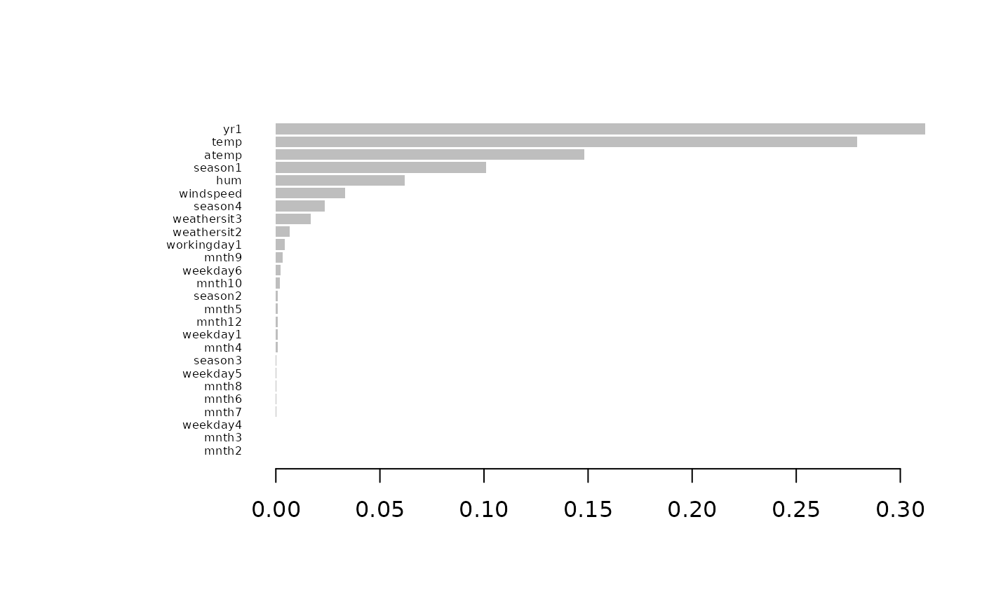

Build a rough model

Let’s sculpt this xgboost model.

Firstly, we need to define a prediction function that takes data as input and returns predictions based on the trained model (in this case, the xgboost above):

xgb_pred <- function(x) {
  predict(est, newdata = model.matrix(~ . - 1, data = x))
}

Secondly, we need to generate product marginals, a grid of values that is sampled independently per each column from the original dataset. For more detailed information on why we do this, please check out the function documentation.

pm <- sample_marginals(
  dat = df_t[covariates], # generate product marginals based on original training data
  n = 10000, # size of the grid
  seed = 372 # for exact reproducibility
)

Check the dimensionality of the grid: number of rows is 10000 as requested, number of columns is the same as the number of covariates.

dim(pm)
#> [1] 10000    11

We will sculpt the model using the generated product marginals:

rough_sculpture <- sculpt_rough(
  dat = pm,
  model_predict_fun = xgb_pred,
  n_ice = 10, # number of ICE curves - increasing this number may increase the stability of the sculpture
  seed = 5 # for exact reproducibility
)

The returned object is a (nested) list of used features with a couple of elements for each feature:

print(rough_sculpture)
#> Rough sculpture with 11 variables
print(typeof(rough_sculpture))
#> [1] "list"
print(str(rough_sculpture, 1))
#> List of 11
#>  $ season    :List of 7
#>  $ yr        :List of 7
#>  $ mnth      :List of 7
#>  $ holiday   :List of 7
#>  $ weekday   :List of 7
#>  $ workingday:List of 7
#>  $ weathersit:List of 7
#>  $ temp      :List of 7
#>  $ atemp     :List of 7
#>  $ hum       :List of 7
#>  $ windspeed :List of 7
#>  - attr(*, "offset")= num 4510
#>  - attr(*, "class")= chr [1:3] "rough" "sculpture" "list"
#>  - attr(*, "var_imp")=Classes 'data.table' and 'data.frame': 11 obs. of  4 variables:
#>   ..- attr(*, ".internal.selfref")=<externalptr> 
#>  - attr(*, "cumul_R2")=Classes 'data.table' and 'data.frame':    11 obs. of  2 variables:
#>   ..- attr(*, ".internal.selfref")=<externalptr> 
#>  - attr(*, "range")=Classes 'data.table' and 'data.frame':   11 obs. of  2 variables:
#>   ..- attr(*, ".internal.selfref")=<externalptr> 
#> NULL

Let’s display the ICE and PDP curves to understand how the individual features influence the model:

ip <- g_ice(rough_sculpture)

ip$continuous + ggplot2::theme(text = ggplot2::element_text(size = 15))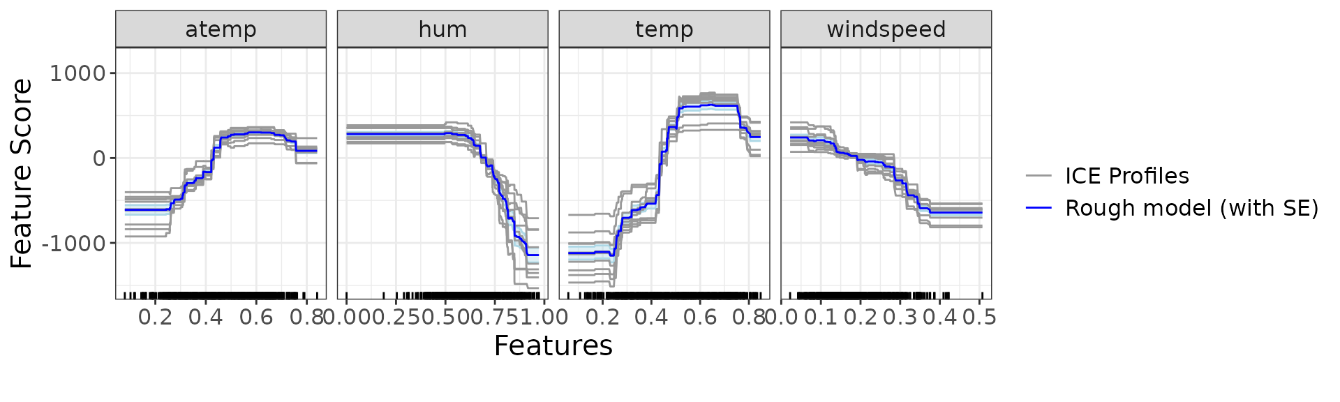

ip$discrete + ggplot2::theme(text = ggplot2::element_text(size = 15))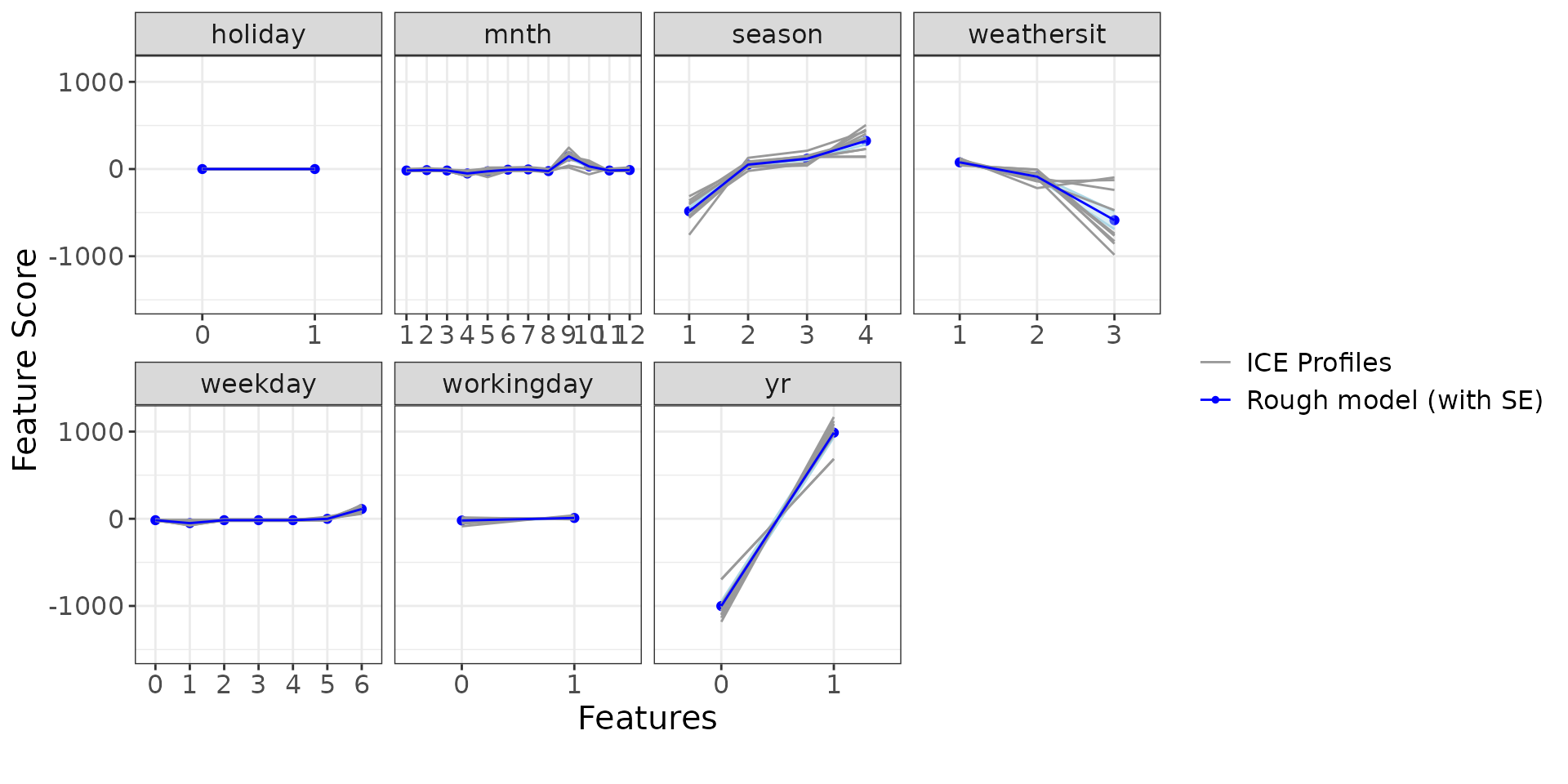

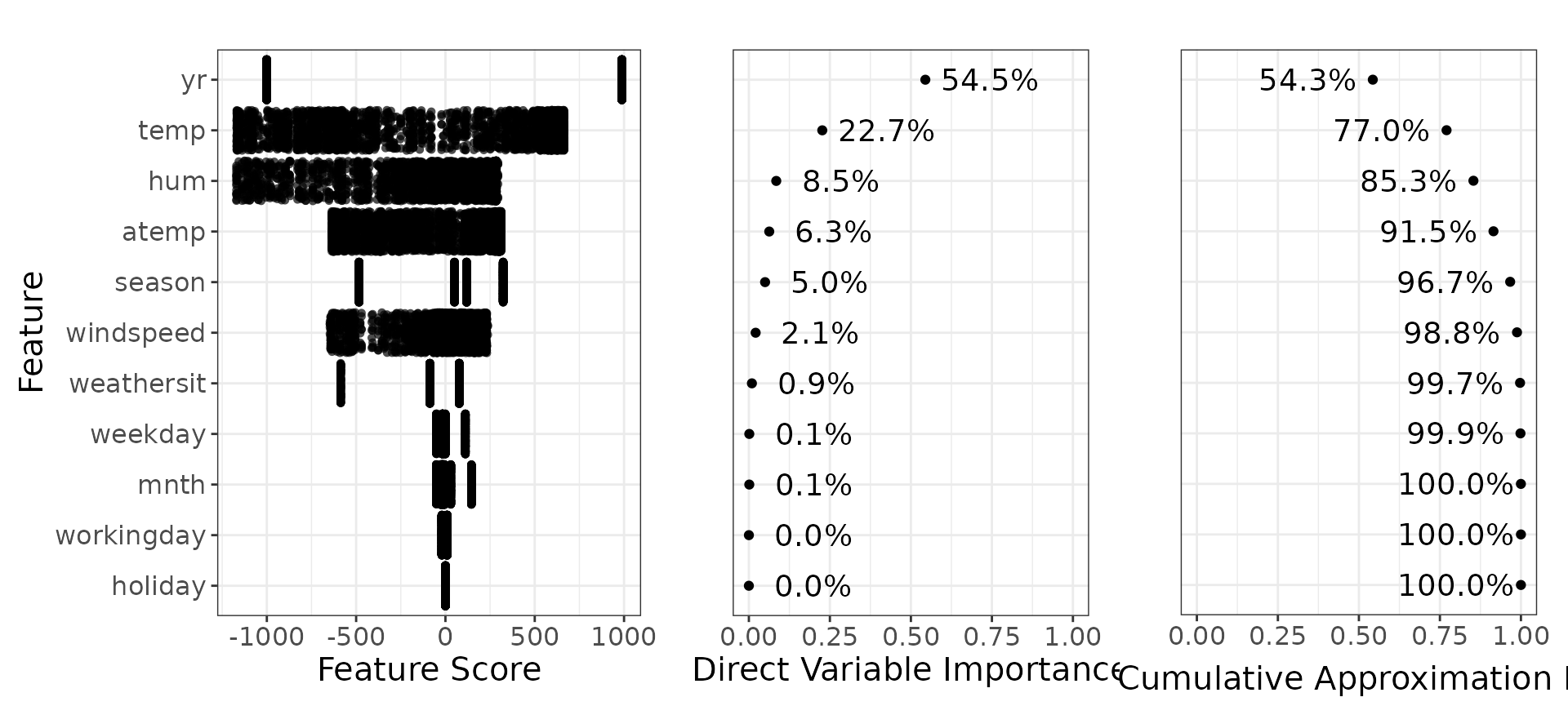
We would also like to see the direct variable importance, a quantity that we have defined in model sculpting. It can be interpreted as feature importance based on the provided model

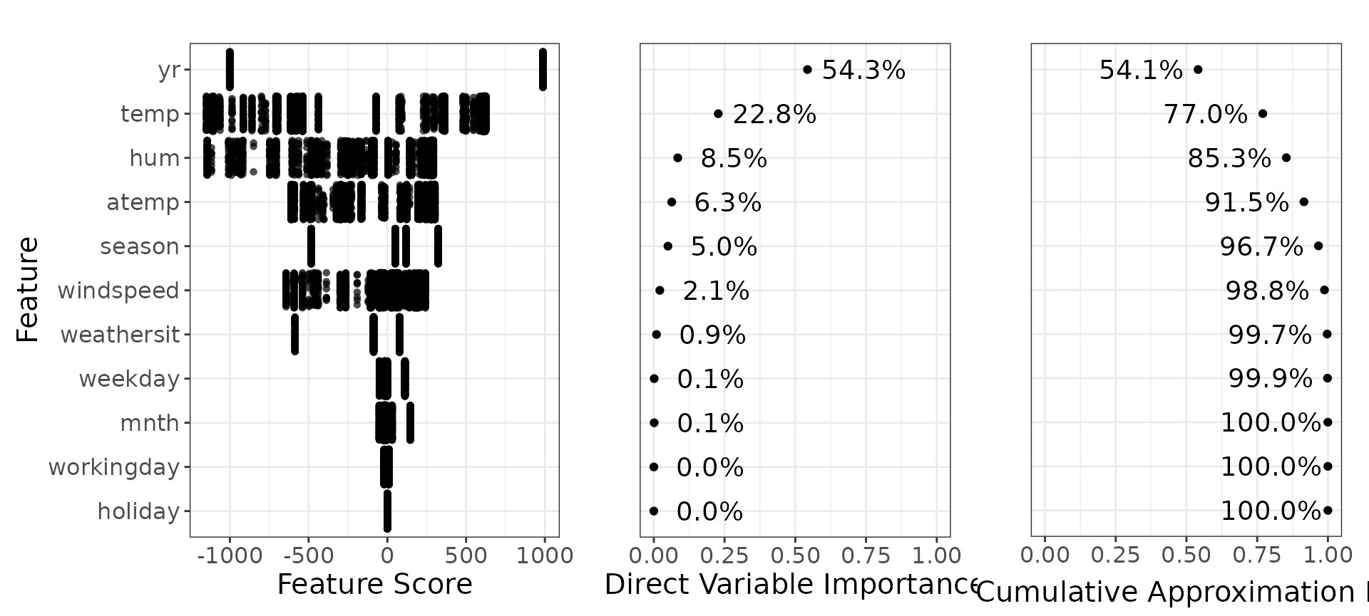
vip <- g_var_imp(rough_sculpture, textsize = 15)
grid::grid.draw(vip)

You can compare this with the variable importances generated by the xgboost.

Build a detailed model

The next step in model sculpting is to smooth the individual PDP curves. This ensures more clear interpretation of the sculpted results. This model we call a detailed model.

You can freely choose which smoothers you would like to use, but you need to write your own function for that. So far, we have prepared two versions: linear models (using lm) and generalized additive models (using mgcv::gam with smoothness).

Detailed model using lm smoother

Let’s start with a linear smoother We create a detailed model using lm smoother based on the rough model above:

detailed_sculpture_lm <- sculpt_detailed_lm(rough_sculpture)

Let’s have a look at the results.

dsp_lm <- g_component(detailed_sculpture_lm)

dsp_lm$continuous + ggplot2::theme(text = ggplot2::element_text(size = 15))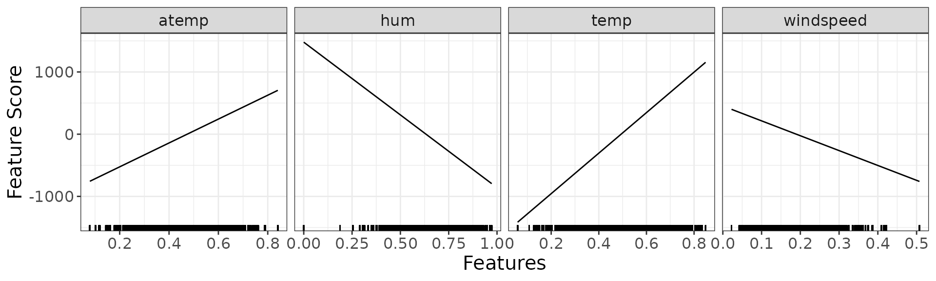

dsp_lm$discrete + ggplot2::theme(text = ggplot2::element_text(size = 15))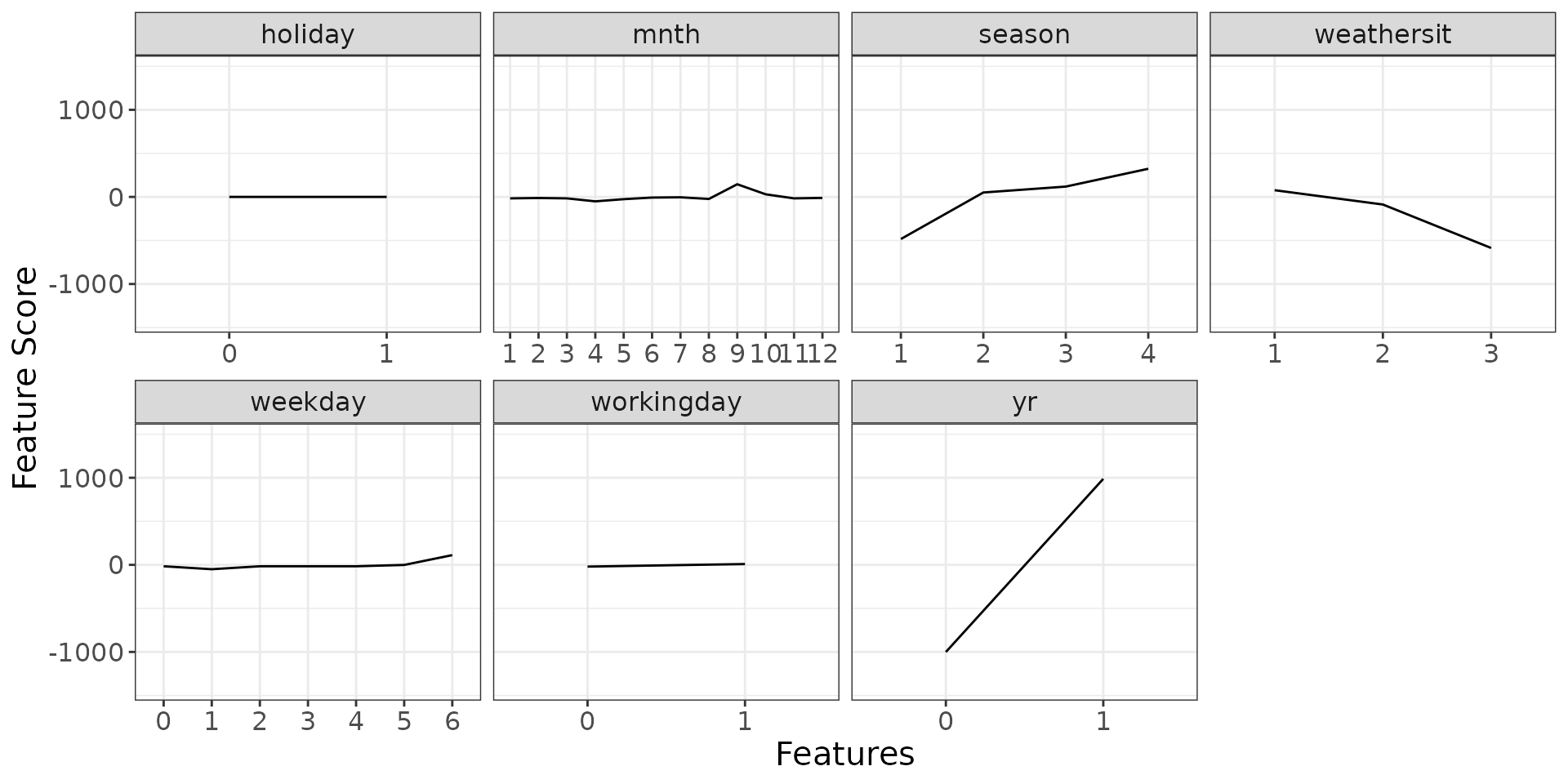

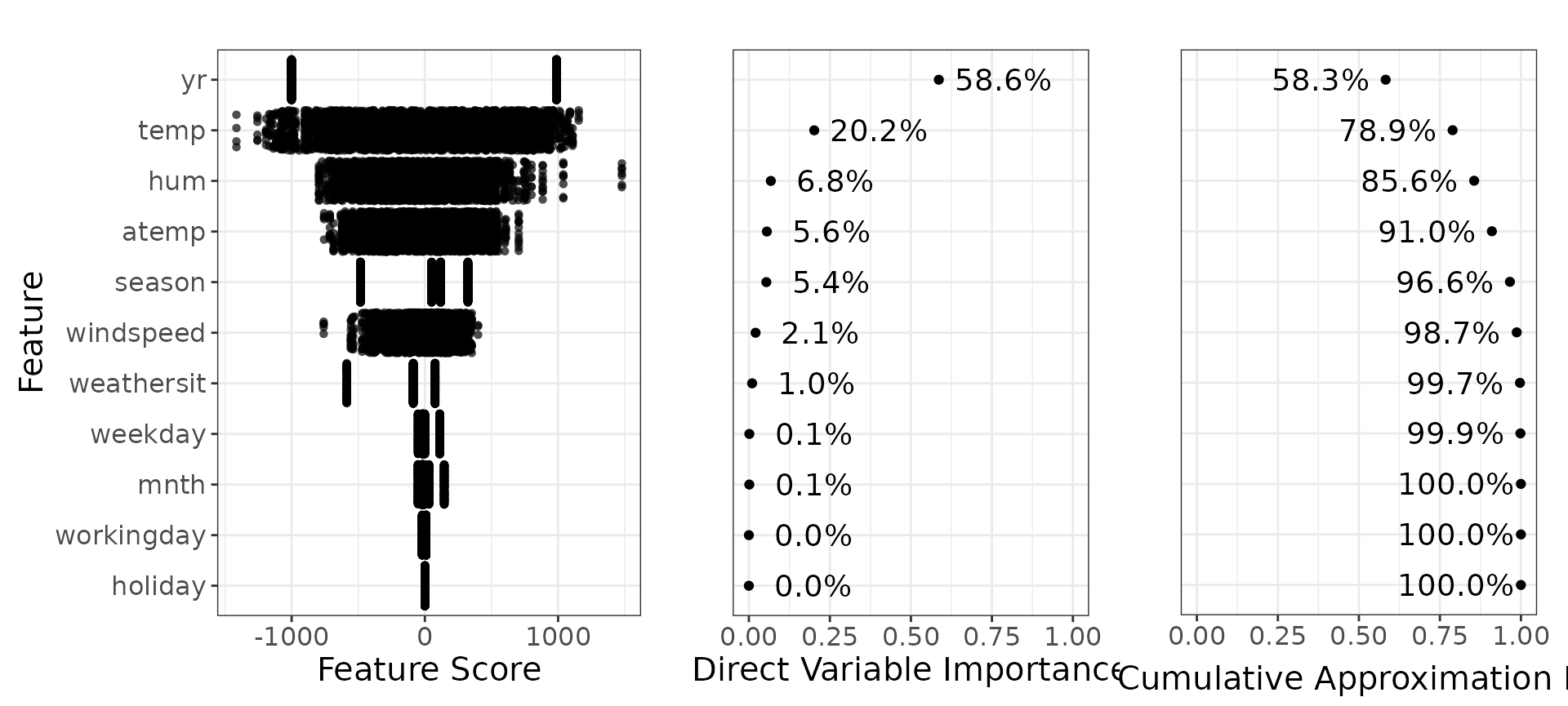
We also show the direct variable importance for this detailed sculpture with lm smoother. Remember to use the product marginals when analysing direct variable importance.

vip_lm <- g_var_imp(detailed_sculpture_lm, textsize = 15)
grid::grid.draw(vip_lm)

Detailed model using gam smoother

We are going to do the same as above just with a different smoother - using mgcv::gam with smoothness mgcv::s.

detailed_sculpture_gam <- sculpt_detailed_gam(rough_sculpture)
#> Loading required namespace: mgcv

Let’s have a look at the results.

dsp_gam <- g_component(detailed_sculpture_gam)

dsp_gam$continuous + ggplot2::theme(text = ggplot2::element_text(size = 15))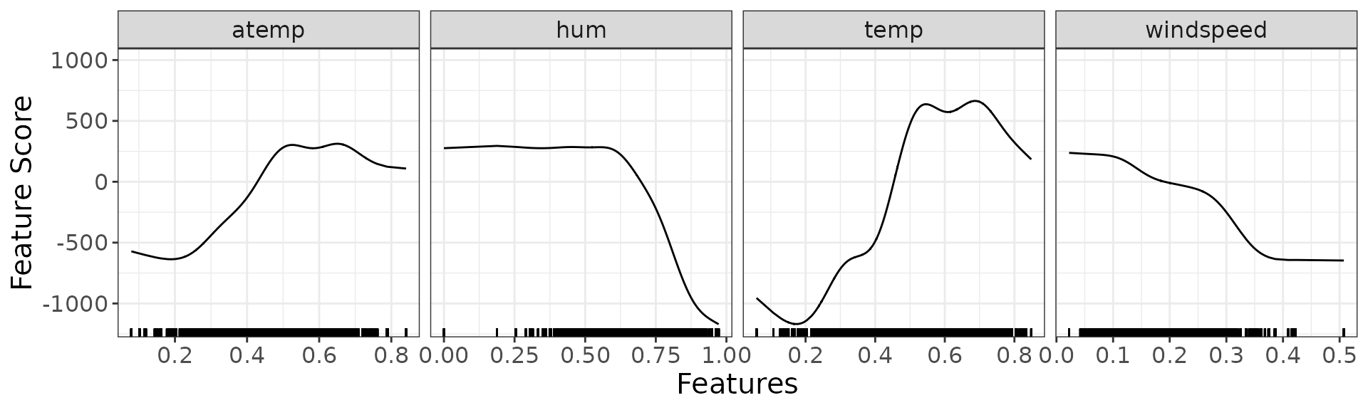

dsp_gam$discrete + ggplot2::theme(text = ggplot2::element_text(size = 15))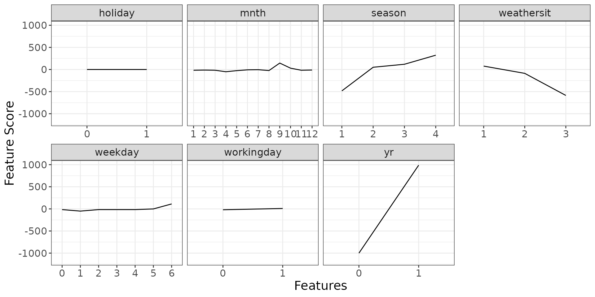

We again show the direct variable importance for this detailed sculpture with gam smoother.

vip_gam <- g_var_imp(detailed_sculpture_gam, textsize = 15)
grid::grid.draw(vip_gam)

Detailed model using arbitrary smoother

You can also define your own arbitrary smoother and build a detailed model on your own.

For that you can use function sculpt_detailed_generic, which works similarly as sculpt_detailed_lm or sculpt_detailed_gam, you just need to provide the definitions of your smoother (parameter smoother_fun) and smoother prediction function (parameter smoother_predict_fun). See the documentation for more info.

Build a polished model

Once we have all the variable importances, we can reduce the model to only a few terms while keeping the highest performance possible. For example, if we decide to go with the detailed model using gam smoothers, and if we aim for at least 95% performance of the original model, we see in the graph above that we can take only yr, temp, season, hum, atemp, windspeed and weathersit features.

polished_sculpture <- sculpt_polished(
  detailed_sculpture_gam,
  vars = c("yr", "temp", "season", "hum", "atemp", "windspeed", "weathersit")
)

length(polished_sculpture) # only 7 out of 11 variables included
#> [1] 7

Compare results

Let’s compare the predictions of the original model vs sculpted models (\(R^2 = 1\) would mean exact match to the xgboost predictions).

g_additivity(
  sp = list(
    predict(rough_sculpture, pm),
    predict(detailed_sculpture_lm, pm),
    predict(detailed_sculpture_gam, pm),
    predict(polished_sculpture, pm)
  ),
  lp = xgb_pred(pm),
  descriptions = c(
    "Rough Model",
    "Detailed model - lm",
    "Detailed model - gam",
    "Polished model"
  ),
  cex = 4
) +
  ggplot2::theme(text = ggplot2::element_text(size = 15))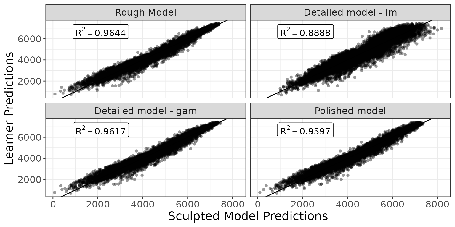

Here we can see the influence of each feature in each of the sculpted model.

scp <- g_comparison(
  sculptures = list(rough_sculpture, detailed_sculpture_lm, detailed_sculpture_gam),
  descriptions = c("Rough", "lm", "gam")
)

scp$continuous + ggplot2::theme(text = ggplot2::element_text(size = 15))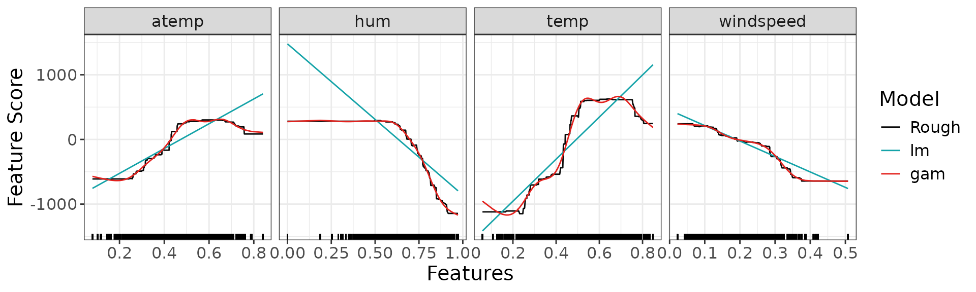

scp$discrete + ggplot2::theme(text = ggplot2::element_text(size = 15))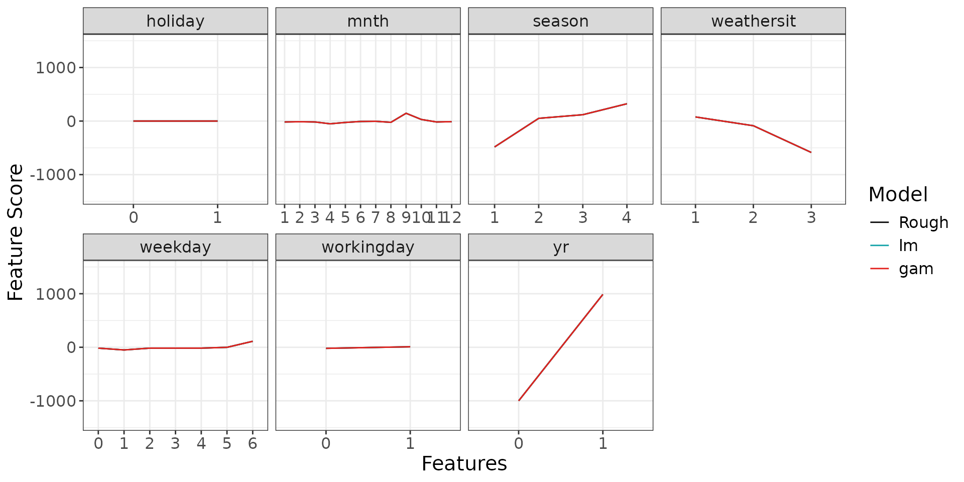

Conclusion

Here we compare the performance of the strong learner with the sculpted models on both train and holdout sets. We will use score_quadratic() and metrics_R2() from the package, which is the traditional coefficient of determination

Train dataset

R2q <- function(y, y_hat) {
  metrics_R2(score_fun = "score_quadratic", y = y, y_hat = y_hat)
}

metrics_train <- data.frame(
  Model = c(
    "Strong learner",
    "Rough model",
    "Detailed model - lm",
    "Detailed model - gam",
    "Polished model"
  ),
  R2 = c(
    R2q(df_t[[response]], xgb_pred(df_t[covariates])),
    R2q(df_t[[response]], predict(rough_sculpture, newdata = df_t[covariates])),
    R2q(df_t[[response]], predict(detailed_sculpture_lm, newdata = df_t[covariates])),
    R2q(df_t[[response]], predict(detailed_sculpture_gam, newdata = df_t[covariates])),
    R2q(df_t[[response]], predict(polished_sculpture, newdata = df_t[covariates]))
  )
)
knitr::kable(metrics_train, align = "lcc")

Model	R2
Strong learner	0.9273318
Rough model	0.8726919
Detailed model - lm	0.7976886
Detailed model - gam	0.8644481
Polished model	0.8603234

Holdout dataset

metrics_test <- data.frame(
  Model = c(
    "Strong learner",
    "Rough model",
    "Detailed model - lm",
    "Detailed model - gam",
    "Polished model"
  ),
  R2 = c(
    R2q(df_h[[response]], xgb_pred(df_h[covariates])),
    R2q(df_h[[response]], predict(rough_sculpture, newdata = df_h[covariates])),
    R2q(df_h[[response]], predict(detailed_sculpture_lm, newdata = df_h[covariates])),
    R2q(df_h[[response]], predict(detailed_sculpture_gam, newdata = df_h[covariates])),
    R2q(df_h[[response]], predict(polished_sculpture, newdata = df_h[covariates]))
  )
)
knitr::kable(metrics_test, align = "lcc")

Model	R2
Strong learner	0.8718544
Rough model	0.8523495
Detailed model - lm	0.7673903
Detailed model - gam	0.8570278
Polished model	0.8505340

Note that the only model with any interaction is the XGBoost (Strong learner), all the other models are purely additive (i.e. without interactions), which are much easier to interpret.

Based on the results above, it seems that removing the interaction lowers the performance only slightly. Depending on the use case, it may be better to use the less complex and more interpretable polished model than the original strong learner.

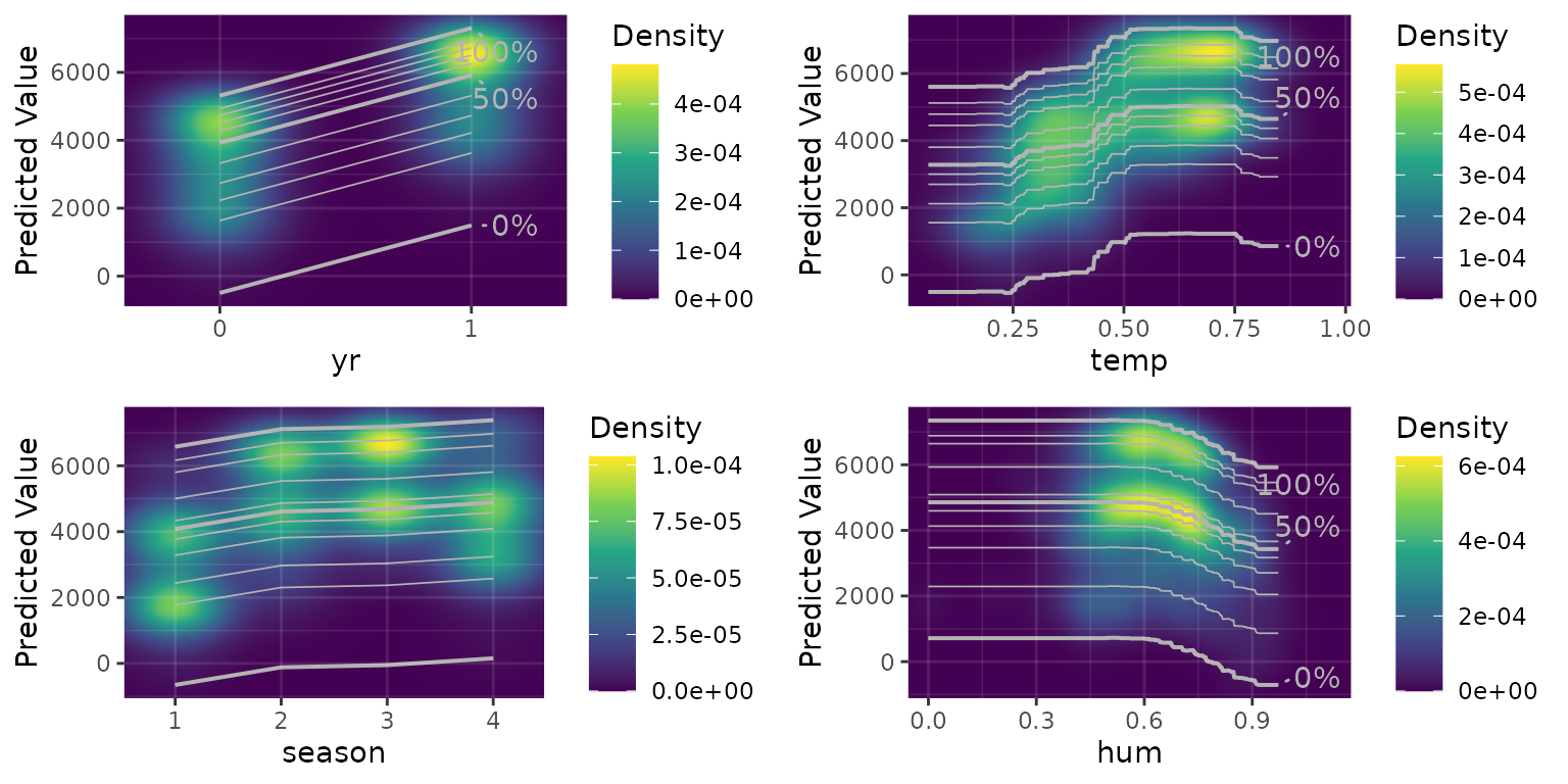
Density plot

The package also has functionality to visualize where the data were located when the model was trained.

density_plots <-
  g_density_ice_plot_list(rough_sculpture, df_t,
    c("yr", "temp", "season", "hum", "atemp", "windspeed", "weathersit"),
    task = "regression"
  )

grid::grid.draw(
  gridExtra::arrangeGrob(
    grobs = density_plots[c("yr", "temp", "season", "hum")]
  )
)