Binary Response • modsculpt

Introduction

Here we will show how to apply model sculpting for a binary endpoint.

library(modsculpt)

Data preparation

Download compas_test.csv and compas_train.csv at https://github.com/corels/corels/tree/master/data and read it in R.

You can use the following code to do this:

train <- read.csv("https://raw.githubusercontent.com/corels/corels/master/data/compas_train.csv")
test <- read.csv("https://raw.githubusercontent.com/corels/corels/master/data/compas_test.csv")

In this dataset, recidivate.within.two.years is the binary response that we want to predict, the other columns are features.

response <- "recidivate.within.two.years"
covariates <- c("sex", "age", "juvenile.felonies", "juvenile.misdemeanors", "juvenile.crimes", "priors", "current.charge.degree")

All of the features are factors so let’s convert them:

train[covariates] <- lapply(train[covariates], as.factor)
# reorder levels
levels(train$priors) <- c("=0", "=1", "2-3", ">3")
levels(train$age) <- c("18-20", "21-22", "23-25", "26-45", ">45")

test[covariates] <- lapply(test[covariates], as.factor)
# reorder levels
levels(test$priors) <- c("=0", "=1", "2-3", ">3")
levels(test$age) <- c("18-20", "21-22", "23-25", "26-45", ">45")

Model Sculpting

Build a base model

Firstly, check the NAs:

anyNA(train)
#> [1] FALSE

Secondly, check zero variance columns (all columns are factors):

any(sapply(train, \(x) length(unique(x)) == 1))
#> [1] FALSE

Now let’s build a strong learner via xgboost (again with already predefined parameters):

requireNamespace("xgboost")
#> Loading required namespace: xgboost
set.seed(567)
est <- xgboost::xgb.train(
  params = list(
    booster = "gbtree",
    objective = "binary:logistic",
    eta = 0.03,
    gamma = 0.75,
    max_depth = 2,
    min_child_weight = 15,
    colsample_bytree = 1,
    subsample = 0.5
  ),
  nrounds = 100,
  data = xgboost::xgb.DMatrix(
    data = model.matrix(~ . - 1, data = train[covariates]),
    label = train[[response]]
  ),
  verbose = 0,
  nthread = 2
)

Here you can see the variable importances based on xgboost:

xgboost::xgb.plot.importance(xgboost::xgb.importance(model = est))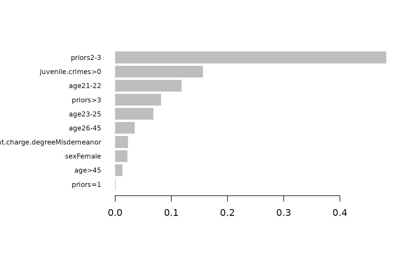

Build a rough model

Let’s sculpt this xgboost model.

Firstly, we need to define a prediction function that takes data as input and returns predictions based on the trained model (in this case, the xgboost above).

For a binary response, it is worth to sculpt the model on the log-odds scale instead of the probability scale since the xgboost is built in the log-odds scale as well (see parameter objective = "binary:logistic").

xgb_pred <- function(x) {
  probs <- predict(est, newdata = model.matrix(~ . - 1, data = x))
  log(probs / (1 - probs)) # convert to log of odds
}

Secondly, we need to generate product marginals, a grid of values that is sampled independently per each column from the original dataset.

pm <- sample_marginals(
  dat = train[covariates], # generate product marginals based on original training data
  n = 10000, # size of the grid
  seed = 372 # for exact reproducibility
)

We will sculpt the model using the generated product marginals:

rough_sculpture <- sculpt_rough(
  dat = pm,
  model_predict_fun = xgb_pred,
  n_ice = 10, # number of ICE curves - increasing this number may increase the stability of the sculpture
  seed = 5 # for exact reproducibility
)

Let’s display the ICE and PDP curves to understand how the individual features influence the model. Remember that y-axis (“Feature Score”) describes the log of odds.

ip <- g_ice(rough_sculpture)

ip$discrete + ggplot2::theme(text = ggplot2::element_text(size = 15))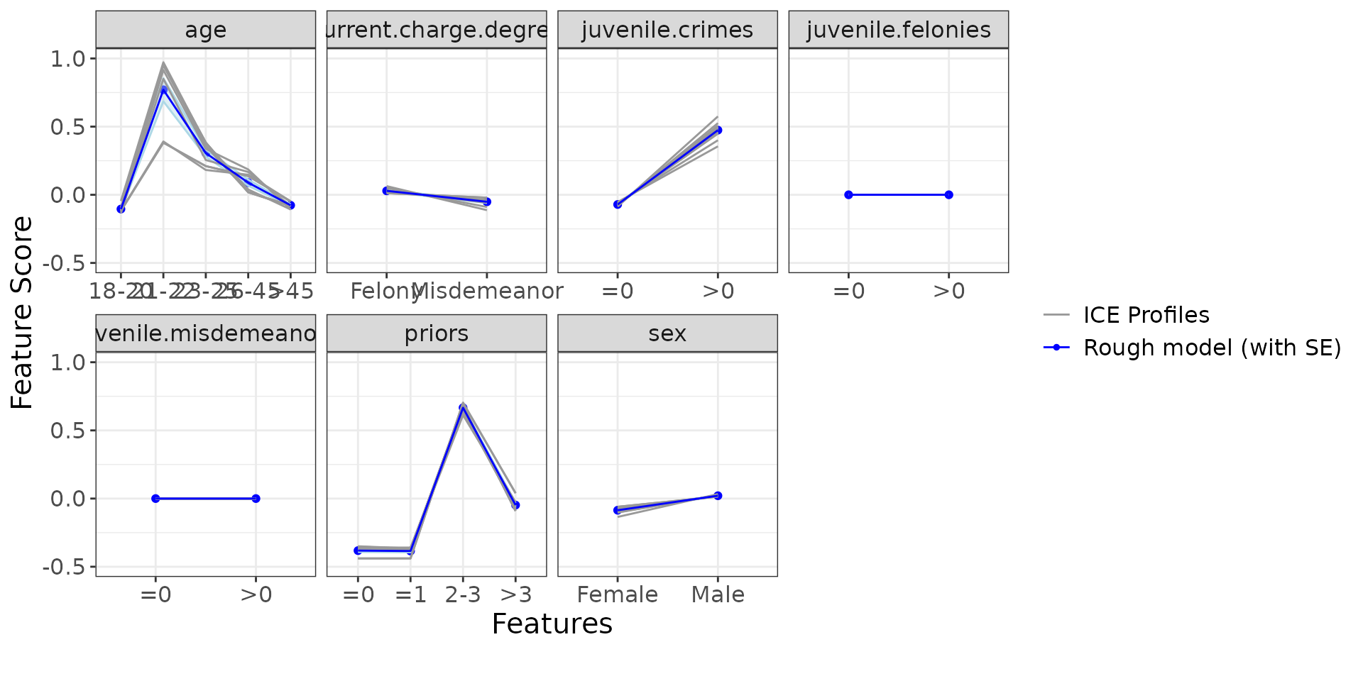

Below we can see the direct variable importance:

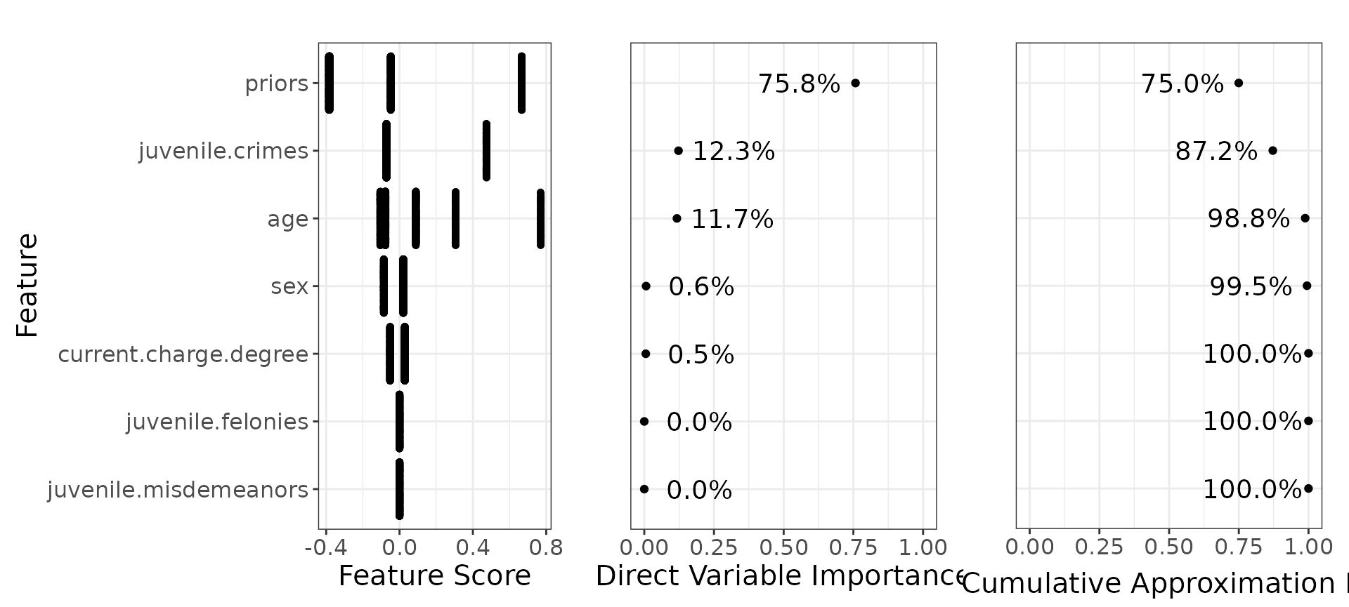
vip <- g_var_imp(rough_sculpture, textsize = 15)
grid::grid.draw(vip)

You can compare this with the variable importances generated by the xgboost.

Build a polished model

Let’s jump to polished model now, using only the top 4 features:

polished_sculpture <- sculpt_polished(
  rough_sculpture,
  vars = c("priors", "juvenile.crimes", "age", "sex")
)

Compare results

Let’s compare the predictions of the original model vs sculpted models (\(R^2 = 1\) would mean exact match to the xgboost predictions).

g_additivity(
  sp = list(predict(rough_sculpture, pm), predict(polished_sculpture, pm)),
  lp = xgb_pred(pm),
  descriptions = c("Rough Model", "Polished model"),
  cex = 4
) +
  ggplot2::theme(text = ggplot2::element_text(size = 15))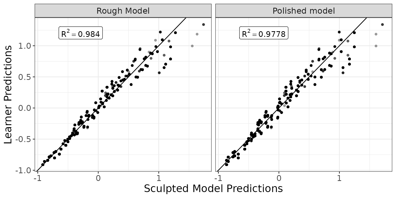

Test dataset

Finally, below we compare the performance of the model (using quadratic loss):

R2q <- function(y, y_hat) {
  metrics_R2(score_fun = "score_quadratic", y = y, y_hat = y_hat)
}

Remember that the predictions refer to the log of odds. To convert this to probabilities, we need to transform them:

inv.logit <- function(x) 1 / (1 + exp(-x))

metrics_test <- data.frame(
  Model = c(
    "Strong learner",
    "Rough model",
    "Polished model"
  ),
  R2 = c(
    R2q(test[[response]], inv.logit(xgb_pred(test[covariates]))),
    R2q(test[[response]], inv.logit(predict(rough_sculpture, newdata = test[covariates]))),
    R2q(test[[response]], inv.logit(predict(polished_sculpture, newdata = test[covariates])))
  )
)
knitr::kable(metrics_test, align = "lc")

Model	R2
Strong learner	0.1604679
Rough model	0.1598891
Polished model	0.1571700

Since the “Strong learner” is the only model with interactions, the table above suggests that the interactions are not significant as the performance of the “Rough model” is almost the same.

What is more, using the “Polished model” with only 4 selected features further reduces the model complexity without any significant performance loss.