Fibrosis-associated macrophage in vitro query and comparisons

The goal of this demo is to familiarize users with a couple of SCimilarity’s more flexible functionalities. The application is to fibrosis-associated macrophages (FM\(\phi\)) and loosely parallels much of the FM\(\phi\) analysisfor Figure 6 from the SCimilarity manuscript.

System requirements:

• At least 64GB of RAM

0. Required software and data

Things you need for this demo:

0. SCimilarity package should already be installed.

1. SCimilarity trained model. Download SCimilarity models. Note, this is a large tarball - downloading and uncompressing can take a several minutes.

2. Query data. We will use Adams et al., 2020 healthy and IPF lung scRNA-seq data. Download tutorial data.

For instructions on how to download the demo data or SCimilarity models please check the cell search tutorial.

import scanpy as sc
import numpy as np
import pandas as pd

sc.set_figure_params(dpi=100)

import warnings

warnings.filterwarnings("ignore")

adams = sc.read("/data/GSE136831_subsample.h5ad")

1. Identify query population

from scimilarity.utils import lognorm_counts
from scimilarity import CellQuery, align_dataset, Interpreter

Import SCimilarity - Cell annotation object

# Instantiate the CellQuery object
# Set model_path to the location of the uncompressed model
model_path = "/models/model_v1.1"
cq = CellQuery(model_path)

SCimilarity pre-processing

Note, this section is largely repeat of the SCimilarity pre-processing section from the cell search tutorial.

SCimilarity requires new data to be processed in a specific way that matches how the model was trained.

Match feature space with SCimilarity models

SCimilarity’s gene expression ordering is fixed. New data should be re-orderd to match that. Genes that are not present in the new data will be zero filled to comply to the expected structure. Genes that are not present in SCimilarity’s gene ordering will be filtered out.

Note, SCimilarity was trained with high data dropout to increase robustness to differences in gene lists.

adams = align_dataset(adams, cq.gene_order)

Normalize data consistent with SCimilarity

It is important to match Scimilarity’s normalization so that the data matches the lognorm tp10k procedure used during model training.

adams = lognorm_counts(adams)

With these simple steps, the data is now ready for SCimilarity. We are able to filter cells later (even after embedding) because SCimilarity handles each cell indepdendently and can skip highly variable gene selection altogether.

Identify query cell state

As in the SCimilarity manuscript, we use a signature to identify the cells you want to query. There are many other ways to select a query cell state such as granular clustering and looking at expression patterns of a specific gene.

fm_basic_signature = ["SPP1", "TREM2", "GPNMB", "MMP9", "CHIT1", "CHI3L1"]
sc.tl.score_genes(adams, fm_basic_signature)

Determine query profile

We will query on the centroid of the top n cells that score on our signature.

Select the top scoring cells to define our query cell state

To identify similar cells, we input a query profile representing the cell state of interest. In this case, we will use the average expression profile of cells above the 99.9th percentile of our signature score.

Note, an overly broad cell selection can limit query results.

sig_query_threshold = adams.obs.score.quantile(0.999)
cells_used_in_query = adams.obs.score >= sig_query_threshold
adams.obs["used_in_query"] = cells_used_in_query

Compute centroid of top scoring cells and compute embedding

from scimilarity.utils import get_centroid

avg_cell = get_centroid(adams.layers["counts"][adams.obs["used_in_query"]])
avg_embedding = cq.get_embeddings(avg_cell)

FM\(\phi\) Signature derivation

One can use SCimilarity to create a signature using cells from many datasets (e.g., cell search results). Here, for simplicity, we will derive a signature from a single dataset using a cell state predefined with a signature. Typically, users would derive a signature for a new cell state (maybe defined through querying a specific cell cluster) using expression profiles across many datasets.

To derive this signature with SCimilarity, we will compare gene expression profiles (not embeddings directly, although the attribution method uses SCimilirty embeddings) between two populations of cells, the positive set and the negative set. Here our positive set will be our high signature scoring cells and our negative set will be all other cells. The results will show the original input signature as well as addition genes associated with the FM\(\phi\) cell state.

Select cell sets to compare

pos = adams[adams.obs.score >= sig_query_threshold]
neg = sc.pp.subsample(
    adams[adams.obs.score < sig_query_threshold],
    n_obs=len(pos),
    random_state=0,
    copy=True,
)

Use SCimilarity to compare selected cell sets

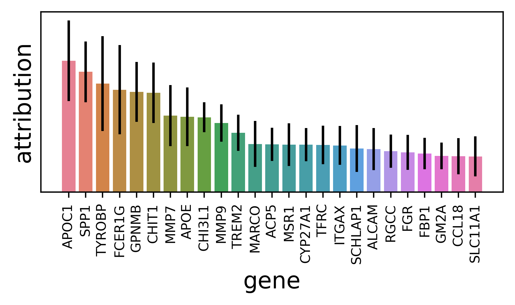
This computes an attribution score and standard deviation for each gene. The more cells used to compute the signature, the lower the standard deviation.

explainer = Interpreter(cq.model, cq.gene_order)
attrs = explainer.get_attributions(pos.X, neg.X)
attrs_df = explainer.get_ranked_genes(attrs)

Visualize genes

While scores are computed for all genes, we will visualize just the top 25. attrs_df is already sorted by attribution and we can show the standard deviation atop that to display uncertainty.

explainer.plot_ranked_genes(attrs_df, n_plot=25)

Note, because we are working off of neural network gradients, we don’t have an intuitive understanding of the scale of attribution values. Therefore, we try to avoid quantititavely interpreting them and instead focus on the attribution values relative to other genes within the same comparison.

2. Pairwise distance to all in vitro macrophages

Get all metadata, identify predicted macrophages

meta = cq.cell_metadata

SCimilarity models contain all cell and sample metadata - an extremely valuable resource

Each row corresponds to the metadata for one cell. Use it to filter results based on cell type, tissue, disease, in vitro, etc.

# Show a random sampling of 5 annotations
meta.sample(5)

	index	study	sample	prediction	fm_signature_score	n_genes_by_counts	total_counts	total_counts_mt	pct_counts_mt	prediction_nn_dist	...	cell_line	iPSC-derived	ESC-derived	xenograft	tissue	cell_line_cleaned	disease	FACS_sort	sex_cleaned	author_label
22934587	22934587	DS000011735	DS000011735-GSM4058930	alveolar macrophage	-0.239148	1187.0	2471.0	126.0	5.099150	1.514161e-02	...	False	NA	NA	NA	lung	NA	chronic obstructive pulmonary disease	NA	NA	alveolar macrophage
12004876	12004876	ENCODE	ENCFF616DEQ	macrophage	-0.103378	849.0	1141.0	11.0	0.964067	1.489848e-02	...	False	False	False	False	heart left ventricle	NA	NA	NA	NA	NA
20933434	20933434	436154da-bcf1-4130-9c8b-120ff9a888f2	a95f8d98-ff4e-45fc-8ede-1687c1495833	CD4-positive, alpha-beta T cell	0.000000	559.0	1699.0	40.0	2.354326	-2.384186e-07	...	False	NA	NA	NA	blood	NA	systemic lupus erythematosus	NA	NA	CD4-positive, alpha-beta T cell
5533835	5533835	GSE136394	GSM4047948	CD4-positive, alpha-beta T cell	0.000000	2190.0	5904.0	309.0	5.233740	7.584751e-03	...	False	False	False	False	NA	NA	colorectal cancer	NA	NA	NA
11224869	11224869	GSE139829	GSM4147092	melanocyte	-0.011139	1283.0	2769.0	477.0	17.226435	6.371522e-02	...	False	False	False	False	uvea	NA	melanoma	NA	female	NA

5 rows × 25 columns

Extract precomputed embeddings for all macrophages across samples and studies

Filter criteria:

• Must be a macrophage population with >50 macrophages

SCimilarity has built-in Cell Onotology support that the user can import and use in their queries. In this example, we demonstrate the import of monocyte, macrophage and microglia descendants using their ontology and the get_all_descendant() method. We then merge the monocyte and macrophage descendants and remove those of the microglia. Using another builtin method get_id_mapper() we map the cell identifiers to their names.

from scimilarity.ontologies import (
    import_cell_ontology,
    get_id_mapper,
    get_all_descendants,
)

# prepare cell ontology
onto = import_cell_ontology(url="http://purl.obolibrary.org/obo/cl/cl-basic.obo")
id2name = get_id_mapper(onto)

mono_descendents = get_all_descendants(onto, "CL:0000576", inclusive=True)
mac_descendents = get_all_descendants(onto, "CL:0000235", inclusive=True)
microglia_descendents = get_all_descendants(onto, "CL:0000129", inclusive=True)

momac_ids = pd.Index((mono_descendents | mac_descendents) - microglia_descendents)
momac_cell_types = momac_ids.map(id2name)

From the metadata of SCimilarity datasets we can then select the relevant cell types. Since our experimental query cells were cultured in vitro we will filter out the cells coming from in vivo experiments.

momac_inds = meta.prediction.isin(momac_cell_types)
in_vitro_inds = (meta["in_vivo"] == "False").values
in_vitro_momac_inds = momac_inds & in_vitro_inds
momac_meta = meta[in_vitro_momac_inds]

Extract pre-computed cell embeddings for in vitro monocytes and macrophages

After identifying the relevant cells we can compute their embedding in the pretrained model. This execution is very fast, extracting over 100k cells from across studies in under 2.5s

%%time
momac_embeddings = cq.get_precomputed_embeddings(np.where(in_vitro_momac_inds)[0])
momac_embeddings.shape

CPU times: user 11.6 s, sys: 3.02 s, total: 14.6 s
Wall time: 3.35 s

(145323, 128)

Compute pairwise distance from query embedding to all other macrophages

We will use the embedding to calculate the distance from query cells to the surrounding cells and calculate their scimilarity as 1/distance.

mac_distances = 1 - (momac_embeddings @ avg_embedding.T).flatten()

momac_meta["distance"] = mac_distances
momac_meta["similarity"] = 1 / mac_distances

momac_meta["sample"] = pd.Categorical(momac_meta["sample"])

We can then narrow the results down to the samples that have a sufficient number of cells (in this example we choose 25 cells).

cell_counts_per_sample = momac_meta.groupby("sample").size()
samples_w_enough_cells = cell_counts_per_sample[cell_counts_per_sample > 25].index
momac_meta = momac_meta[momac_meta["sample"].isin(samples_w_enough_cells)]
momac_meta["sample"] = momac_meta["sample"].cat.remove_unused_categories()

import seaborn as sns
from matplotlib import pyplot as plt

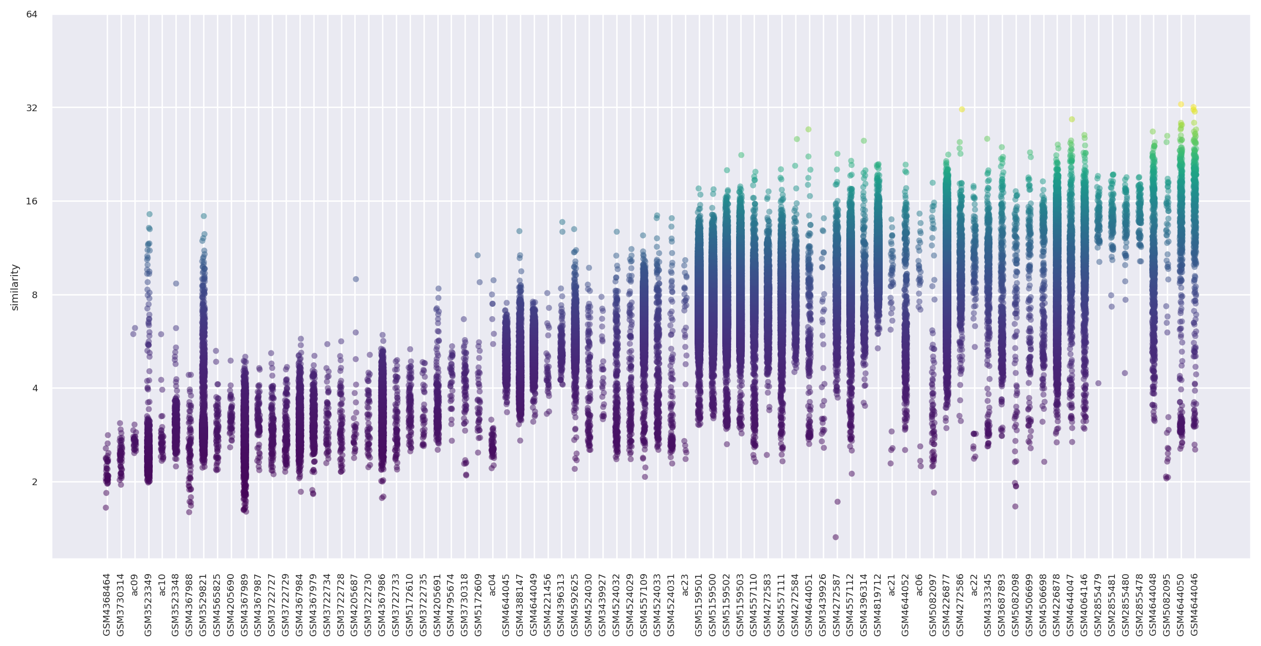
We can plot similarity scores across the relevant studies.

# Disclaimer: this is a somewhat hacky workaround to add jitter to seaborn's scatterplot().
# While stripplot() can do this natively, it's much more resource-hungry.

# 1. Order the categories on the x-axis
sample_order = list(
    momac_meta.groupby("sample")["similarity"].quantile(0.9).sort_values().index
)
momac_meta["sample"] = pd.Categorical(
    momac_meta["sample"], categories=sample_order, ordered=True
)

# 2. Transform the categorical data into numerical values
momac_meta["numeric_sample"] = momac_meta["sample"].cat.codes

# 3. Add jitter (Add more or less jitter depending on the plot by adjust the jitter strength)
jitter_strength = 0.1
momac_meta["jittered_sample"] = momac_meta["numeric_sample"] + np.random.uniform(
    -jitter_strength, jitter_strength, size=len(momac_meta)
)

# 4. Now, plot using the jittered values
sns.set(font_scale=0.6)
plt.figure(figsize=(15, 7))
ax = sns.scatterplot(
    data=momac_meta,
    x="jittered_sample",
    y="similarity",
    hue="similarity",
    palette="viridis",
    linewidth=0,
    size=0.1,
    alpha=0.5,
)

ax.set_yscale("log", base=2)
ax.legend().set_visible(False)
ax.set_yticks([2, 4, 8, 16, 32, 64])
ax.set_yticklabels(["2", "4", "8", "16", "32", "64"])

# Set the x-ticks based on the desired order
ax.set_xticks(range(len(sample_order)))
ax.set_xticklabels(sample_order, rotation=90)
ax.set_xlabel("");

Interpretation

3 of the four top in vitro tissue samples are from the Xu et al. 2022 3D culture system dataset that we highlight in the SCimilarity manuscript.

1. GSM4644046 - samples in 3DCS day05 Donor1

2. GSM4644050 - samples in 3DCS day05 Donor2

4. GSM4644048 - samples in 3DCS day14 Donor1

sample_order[-4:]

['GSM4644048', 'GSM5082095', 'GSM4644050', 'GSM4644046']

At this point, we reccomend downloading the datasets and looking into the experimental design to explore the implications that these new conditions may have on your hypothesis!