Annotating cell types#
This tutorial is to familiarize users with SCimilarity’s basic cell annotation functionality.
System requirements:
At least 64GB of RAM
0. Required software and data#
Things you need for this demo:
SCimilarity package should already be installed.
SCimilarity trained model. Download SCimilarity models. Note, this is a large tarball - downloading and uncompressing can take a several minutes.
A dataset to annotate. We will use Adams et al., 2020 healthy and IPF lung scRNA-seq data. Download tutorial data.
If the model hasn’t been downloaded please uncomment and run the two command below
[1]:
# !curl -L -o /models/model_v1.1.tar.gz \
#   https://zenodo.org/records/10685499/files/model_v1.1.tar.gz?download=1
# !tar -xzvf /models/model_v1.1.tar.gz
If the data hasn’t been downloaded please uncomment and run the two command below
[2]:
# !curl -L -o "/data/GSE136831_subsample.h5ad" \
#   https://zenodo.org/records/13685881/files/GSE136831_subsample.h5ad?download=1
[3]:
import scanpy as sc
from matplotlib import pyplot as plt

import warnings
warnings.filterwarnings("ignore")
[4]:
sc.set_figure_params(dpi=100)
sc.settings.verbosity = 0
plt.rcParams["figure.figsize"] = [6, 4]
plt.rcParams["pdf.fonttype"] = 42
from scimilarity import CellAnnotation
from scimilarity.utils import align_dataset, lognorm_counts
1. Prepare for SCimilarity: Import and normalize data#
[5]:
# Instantiate the CellAnnotation object
# Set model_path to the location of the uncompressed model
model_path = "/models/model_v1.1"
ca = CellAnnotation(model_path=model_path)
Load scRNA-seq data#
[6]:
# Load the tutorial data
# Set data_path to the location of the tutorial dataset
data_path = "/data/GSE136831_subsample.h5ad"
adams = sc.read(data_path)
SCimilarity pre-processing#
SCimilarity requires new data to be processed in a specific way that matches how the model was trained.
Match feature space with SCimilarity models#
SCimilarity’s gene expression ordering is fixed. New data should be reorderd to match that, so that it is consistent with how the model was trained. Genes that are not present in the new data will be zero filled to comply to the expected structure. Genes that are not present in SCimilarity’s gene ordering will be filtered out.
Note, SCimilarity was trained with high data dropout to increase robustness to differences in gene lists.
[7]:
adams = align_dataset(adams, ca.gene_order)
Normalize data consistent with SCimilarity#
It is important to match Scimilarity’s normalization so that the data matches the lognorm tp10k procedure used during model training.
[8]:
adams = lognorm_counts(adams)
With these simple steps, the data is now ready for SCimilarity. We are able to filter cells whenever we want (even after embedding) because SCimilarity handles each cell independently and can skip highly variable gene selection altogether.
2. Compute embeddings#
Using the already trained model, SCimilarity can embed your new dataset.
[9]:
adams.obsm["X_scimilarity"] = ca.get_embeddings(adams.X)
Compute visualization of embeddings#
Use UMAP to visualize SCimilarity embeddings#
[10]:
sc.pp.neighbors(adams, use_rep="X_scimilarity")
sc.tl.umap(adams)
Visualize author annotations on the SCimilarity embedding#
[11]:
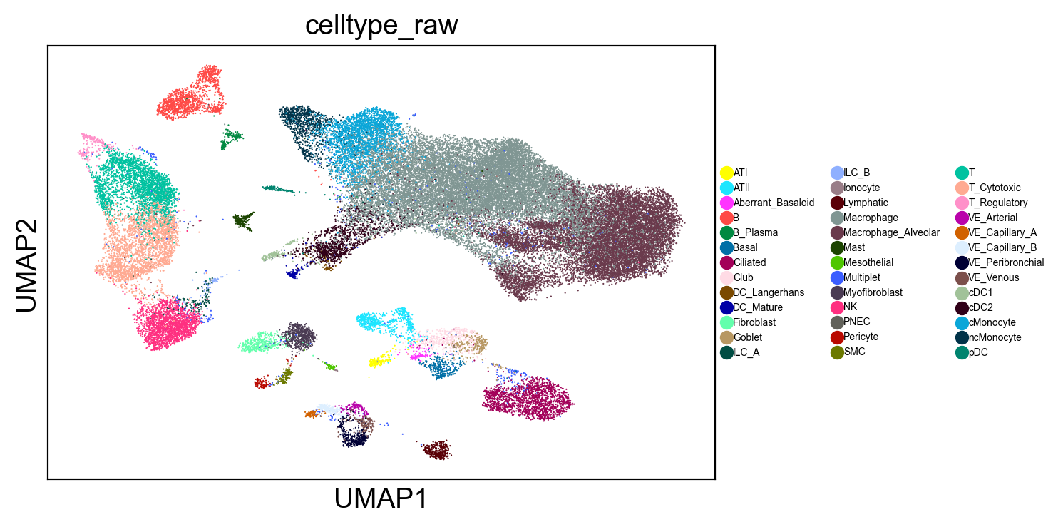
sc.pl.umap(adams, color="celltype_raw", legend_fontsize=5)
plt.savefig("adams_umap.png", dpi=300, bbox_inches="tight")
<Figure size 600x400 with 0 Axes>
Given that author annotations are derived from a different analysis, seeing author annotations roughly cluster in SCimilarity embedding space gives us confidence in our representation. The Adams et al. dataset was not included in the training set, meaning that this is the first time the model has seen this data, yet it is still able to represent the cells present.
3. Cell type classification#
Two methods within the CellAnnotation class:
annotate_dataset- automatically computes embeddings.get_predictions_knn- more detailed control of annotation.
h Description of inputs
X_scimilarity: embeddings from the model, which can be used to generate UMAPs in lieu of PCA and is generalized across datasets.
Description of outputs
predictions: cell type annotation predictions.nn_idxs: indicies of cells in the SCimilarity reference.nn_dists: the minimum distance within k=50 nearest neighbors.nn_stats: a dataframe containing useful metrics such as:hits: the distribution of celltypes in k=50 nearest neighbors.
Unconstrained annotation#
Cells can be classified as any type that is in the SCimilarity reference
[12]:
predictions, nn_idxs, nn_dists, nn_stats = ca.get_predictions_knn(
    adams.obsm["X_scimilarity"], weighting=True
)
adams.obs["predictions_unconstrained"] = predictions.values
Get nearest neighbors finished in: 0.0311508576075236 min
100%|███████████████████████████████████████████████████████████████████████████████████████████████████████████████████████████████████████████████████████████████████████████████████████████████████████████████████████████████████| 50000/50000 [00:20<00:00, 2387.48it/s]
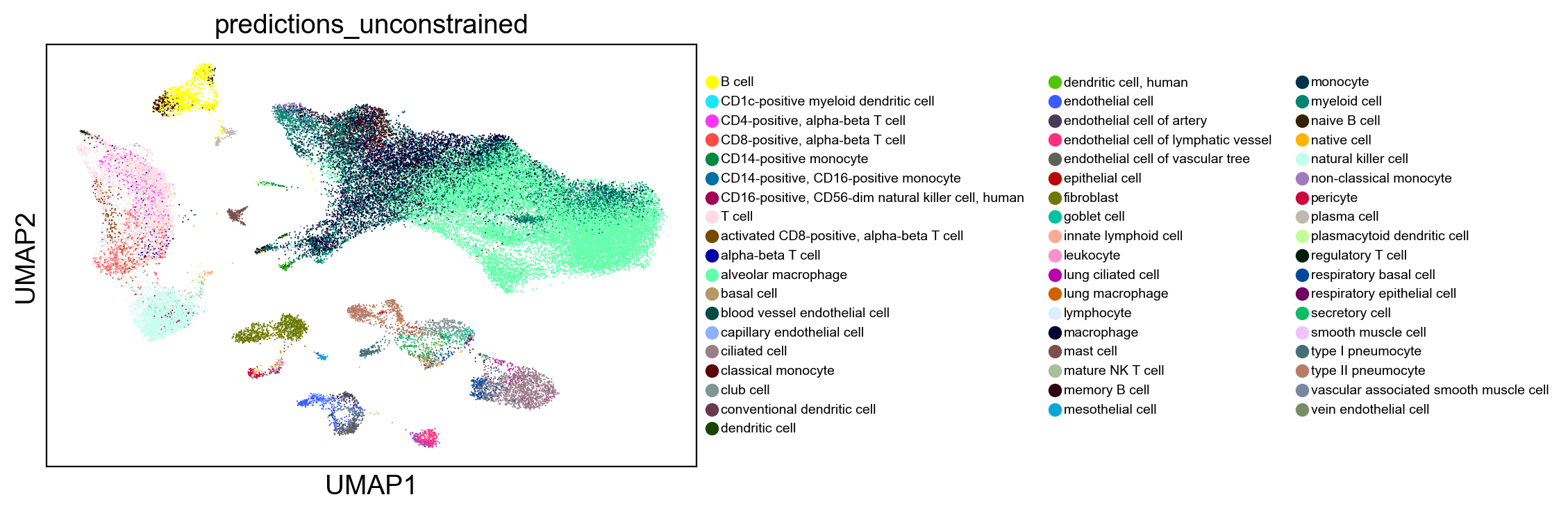
Since each cell is classified independently, there is higher classification noise, filtering out low count cells can reduce the noise in visualization.
[13]:
celltype_counts = adams.obs.predictions_unconstrained.value_counts()
well_represented_celltypes = celltype_counts[celltype_counts > 20].index

sc.pl.umap(
    adams[adams.obs.predictions_unconstrained.isin(well_represented_celltypes)],
    color="predictions_unconstrained",
    legend_fontsize=7,
)
Constrained classification#
By classifying against the full reference, we can get redundant cell types, such as activated CD8-positive, alpha-beta T cell and CD8-positive, alpha-beta T cell.
Alternatively, we can subset the reference to just the cell types we want to classify to. This also reduces noise in cell type annotation.
Note that subsetting can slow classification speeds as the kNN is optimized for the full reference.
[14]:
# We can load all the labels from the model to finetune the labels that we would like to safelist
print("\n".join(ca.classes))
capillary endothelial cell
retinal bipolar neuron
club cell
melanocyte
plasmacytoid dendritic cell
duct epithelial cell
kidney collecting duct principal cell
precursor B cell
luminal cell of prostate epithelium
erythroid lineage cell
inflammatory macrophage
type I pneumocyte
CD14-low, CD16-positive monocyte
neural crest cell
platelet
keratinocyte
oligodendrocyte precursor cell
activated CD4-positive, alpha-beta T cell
double-positive, alpha-beta thymocyte
IgG plasma cell
neural cell
amacrine cell
lymphocyte
pericyte
natural killer cell
CD4-positive, alpha-beta memory T cell
pulmonary ionocyte
CD141-positive myeloid dendritic cell
cholangiocyte
mature NK T cell
enteroendocrine cell
pancreatic ductal cell
regulatory T cell
effector memory CD8-positive, alpha-beta T cell, terminally differentiated
group 3 innate lymphoid cell
blood vessel endothelial cell
dendritic cell, human
vascular associated smooth muscle cell
double negative thymocyte
basal cell
kidney collecting duct intercalated cell
pancreatic acinar cell
mesothelial cell
epithelial cell of proximal tubule
Mueller cell
smooth muscle cell of prostate
leukocyte
endothelial cell of lymphatic vessel
retinal ganglion cell
classical monocyte
intestinal tuft cell
fibroblast
myofibroblast cell
pro-B cell
activated CD8-positive, alpha-beta T cell
lung secretory cell
pancreatic A cell
non-classical monocyte
monocyte
smooth muscle cell
granulocyte
kidney epithelial cell
basal cell of prostate epithelium
mesenchymal stem cell
fat cell
effector memory CD8-positive, alpha-beta T cell
stromal cell
kidney connecting tubule epithelial cell
kidney proximal convoluted tubule epithelial cell
megakaryocyte
CD8-positive, alpha-beta T cell
colon epithelial cell
radial glial cell
lung macrophage
naive T cell
T follicular helper cell
germinal center B cell
interstitial cell of Cajal
pancreatic stellate cell
CD4-positive helper T cell
slow muscle cell
epithelial cell
CD8-positive, alpha-beta memory T cell
mast cell
hepatocyte
respiratory basal cell
hematopoietic stem cell
fast muscle cell
cardiac neuron
conventional dendritic cell
stem cell
gamma-delta T cell
oligodendrocyte
CD16-positive, CD56-dim natural killer cell, human
myeloid cell
myeloid dendritic cell, human
stromal cell of ovary
endothelial cell
paneth cell of epithelium of small intestine
CD16-negative, CD56-bright natural killer cell, human
CD14-positive, CD16-positive monocyte
naive thymus-derived CD4-positive, alpha-beta T cell
follicular dendritic cell
ionocyte
retina horizontal cell
secretory cell
innate lymphoid cell
cardiac muscle cell
enterocyte
class switched memory B cell
respiratory epithelial cell
thymocyte
native cell
alveolar macrophage
mesodermal cell
tracheal goblet cell
plasmablast
medullary thymic epithelial cell
astrocyte
OFF-bipolar cell
kidney loop of Henle thick ascending limb epithelial cell
cardiac endothelial cell
microglial cell
CD4-positive, CD25-positive, alpha-beta regulatory T cell
IgA plasma cell
hematopoietic precursor cell
progenitor cell
glandular epithelial cell
lung neuroendocrine cell
fibroblast of lung
ON-bipolar cell
T cell
periportal region hepatocyte
intestinal crypt stem cell
goblet cell
erythroid progenitor cell
effector memory CD4-positive, alpha-beta T cell
retinal cone cell
retinal rod cell
common lymphoid progenitor
IgM plasma cell
pancreatic D cell
mucosal invariant T cell
T-helper 1 cell
glutamatergic neuron
central memory CD8-positive, alpha-beta T cell
animal cell
neuroendocrine cell
myeloid dendritic cell
parietal epithelial cell
T-helper 17 cell
immature B cell
memory B cell
effector CD4-positive, alpha-beta T cell
memory T cell
neutrophil
CD8-positive, alpha-beta cytotoxic T cell
vein endothelial cell
central memory CD4-positive, alpha-beta T cell
mucus secreting cell
naive regulatory T cell
squamous epithelial cell
fibroblast of cardiac tissue
retinal pigment epithelial cell
mesenchymal cell
lung endothelial cell
type II pneumocyte
naive B cell
CD1c-positive myeloid dendritic cell
CD4-positive, alpha-beta T cell
kidney distal convoluted tubule epithelial cell
bronchial smooth muscle cell
intermediate monocyte
Langerhans cell
naive thymus-derived CD8-positive, alpha-beta T cell
kidney interstitial fibroblast
endothelial cell of vascular tree
plasmacytoid dendritic cell, human
dendritic cell
endothelial cell of hepatic sinusoid
transit amplifying cell of small intestine
enteric smooth muscle cell
macrophage
kidney loop of Henle thin descending limb epithelial cell
B cell
luminal epithelial cell of mammary gland
Kupffer cell
erythrocyte
hepatic stellate cell
type B pancreatic cell
neuron
alpha-beta T cell
CD4-positive, alpha-beta cytotoxic T cell
lung ciliated cell
CD14-positive monocyte
epicardial adipocyte
follicular B cell
glial cell
ciliated cell
paneth cell
effector CD8-positive, alpha-beta T cell
plasma cell
endothelial cell of artery
[15]:
# We will select labels that are relevant to the lung dataset (using our knowledge of the dataset).
# Every user can make their own decision on what labels to safelist depending on the dataset they are analyzing

target_celltypes = [
    "lung macrophage",
    "alveolar macrophage",
    "classical monocyte",
    "non-classical monocyte",
    "conventional dendritic cell",
    "plasmacytoid dendritic cell",
    "mast cell",
    "CD4-positive, alpha-beta T cell",
    "regulatory T cell",
    "CD8-positive, alpha-beta T cell",
    "mature NK T cell",
    "natural killer cell",
    "B cell",
    "plasma cell",
    "type I pneumocyte",
    "type II pneumocyte",
    "club cell",
    "goblet cell",
    "lung ciliated cell",
    "basal cell",
    "respiratory basal cell",
    "secretory cell",
    "neuroendocrine cell",
    "pulmonary ionocyte",
    "endothelial cell of vascular tree",
    "endothelial cell of lymphatic vessel",
    "pericyte",
    "vascular associated smooth muscle cell",
    "fibroblast",
    "myofibroblast cell",
]

ca.safelist_celltypes(target_celltypes)
[16]:
# The ca.annotate_dataset function will now only classify to the safelisted cell types
adams = ca.annotate_dataset(adams)
Get nearest neighbors finished in: 0.09163140455881755 min
100%|███████████████████████████████████████████████████████████████████████████████████████████████████████████████████████████████████████████████████████████████████████████████████████████████████████████████████████████████████| 50000/50000 [00:19<00:00, 2578.92it/s]
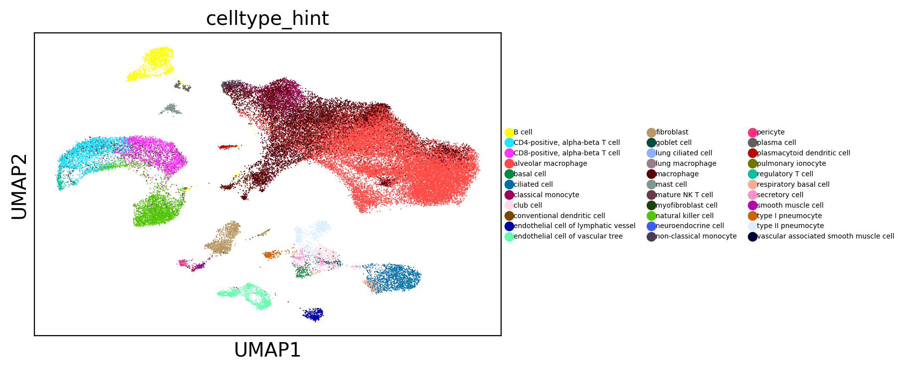
[17]:
sc.pl.umap(adams, color="celltype_hint", legend_fontsize=10)
Annotation QC#
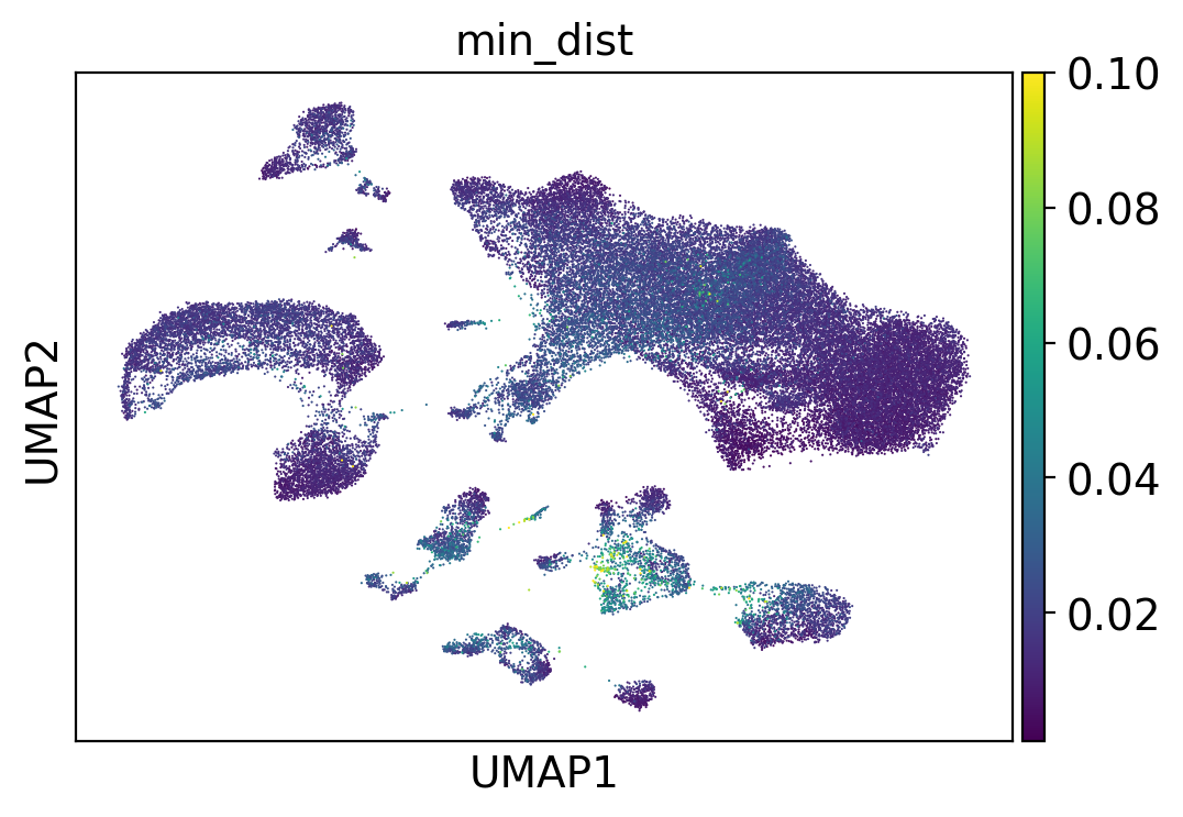
Cell annotation also computes QC metrics for our annotations. One of which, min_dist, represents the minimum distance between a cell in the query dataset and all cells in the training set. The greater min_dist, (i.e., the further away from what the model has seen before) the less confidence we have in the model’s prediction.
Note that for different applications and questions different min_dist ranges have different implications.
The model was trained to push the distance between dissimilar cells (i.e. positive and negative cells in each triplet) to > 0.05 (which is the default margin parameter of the triplet loss function). Distances larger than 0.05 particularly indicate that the model is not confident in the prediction.
[18]:
sc.pl.umap(adams, color="min_dist", vmax=0.1)
plt.savefig("adams_umap_min_dist.png", dpi=300, bbox_inches="tight")
<Figure size 600x400 with 0 Axes>
Alternative method for annotation (cluster consensus annotation)#
An alternative way of performing annotation is to cluster the cells based on the SCimilarity embeddings then use the clusters to predict a single cell type for each cluster. This method is sensitive to the choice of cluster resolution and users are advised to experiment with different resolutions and make sure their clusters are stable and fairly homogenous.
[19]:
sc.tl.leiden(adams, resolution=1)
sc.pl.umap(adams, color="leiden", legend_fontsize=10)
[20]:
# Create leiden-based annotation by picking the most common celltype_hint for each cluster
leiden_based_annotation = {}

# Loop through each unique cluster
for cluster in adams.obs['leiden'].unique():
    # Get all cells in this cluster
    cluster_mask = adams.obs['leiden'] == cluster
    cluster_celltypes = adams.obs.loc[cluster_mask, 'celltype_hint']

    # Find the most common celltype in this cluster
    most_common_celltype = cluster_celltypes.value_counts().index[0]
    leiden_based_annotation[cluster] = most_common_celltype

# Map the cluster-based annotations to all cells
adams.obs['leiden_based_annotation'] = adams.obs['leiden'].map(leiden_based_annotation)
[21]:
# Plot the leiden-based annotation on UMAP
sc.pl.umap(adams, color='leiden_based_annotation', legend_fontsize=10)
We can also visualize the labels within each cluster to troubleshoot some of the problematic clusters
[22]:
import numpy as np
import matplotlib.pyplot as plt

def plot_cluster_label_bars(
    adata,
    cluster_col,
    label_col,
    max_cols=5,
    output_file=None,
    title="Label Counts per Cluster"
):
    unique_clusters = sorted(adata.obs[cluster_col].unique(), key=lambda x: int(x) if str(x).isdigit() else str(x))
    n_clusters = len(unique_clusters)
    n_cols = min(max_cols, n_clusters)
    n_rows = int(np.ceil(n_clusters / n_cols))
    fig, axes = plt.subplots(n_rows, n_cols, figsize=(3.5 * n_cols, 4.5 * n_rows), squeeze=True)

    for idx, cluster in enumerate(unique_clusters):
        row = idx // n_cols
        col = idx % n_cols
        ax = axes[row, col]
        mask = adata.obs[cluster_col] == cluster
        cluster_labels = adata.obs.loc[mask, label_col]
        label_names, counts = np.unique(cluster_labels, return_counts=True)
        ax.bar(label_names, counts)
        ax.set_title(f"Cluster {cluster}")
        ax.set_ylabel("Count")
        ax.set_xticks(range(len(label_names)))
        ax.set_xticklabels(label_names, rotation=45, ha="right", fontsize=10)
        ax.margins(y=0.2)

    for idx in range(n_clusters, n_rows * n_cols):
        row = idx // n_cols
        col = idx % n_cols
        fig.delaxes(axes[row, col])

    fig.suptitle(title, fontsize=20)
    fig.tight_layout(rect=(0, 0, 1, 0.95))
    fig.subplots_adjust(wspace=0.5, hspace=0.8)
    if output_file:
        fig.savefig(output_file, dpi=300, bbox_inches="tight")
    plt.close(fig)

    return fig
[23]:
plot_cluster_label_bars(adams, "leiden", "celltype_hint", max_cols=2, output_file="adams_cluster_label_bars.png")
[23]:
We can see that some of the clusters have more than a single type. It’s up to the users to decide if they are happy with picking the most common label or if they would like to look at these clusters in more detail i.e. subcluster them, plot some canonical gene markers, etc.
Conclusion#
This notebook outlines how to take a dataset and perform cell type annotation.
Keep in mind that the datasets that you analyze with SCimilarity should fit the following criteria:
Data generated from the 10x Genomics Chromium platform (models are trained using this data only).
Human scRNA-seq data.
Counts normalized with SCimilarity functions or using the same process. Different normalizations will have poor results.
[ ]: