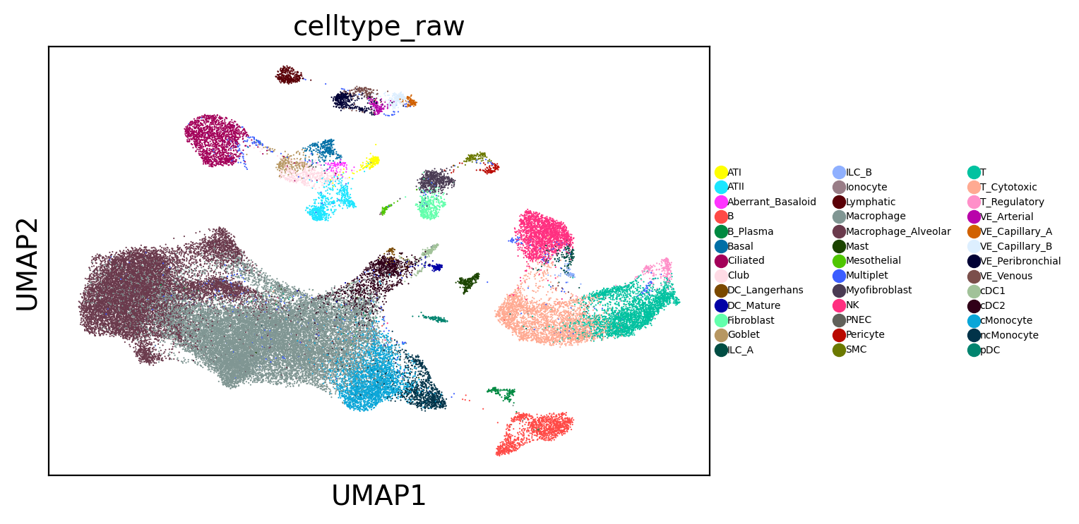
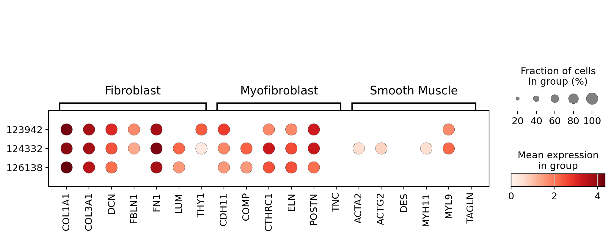
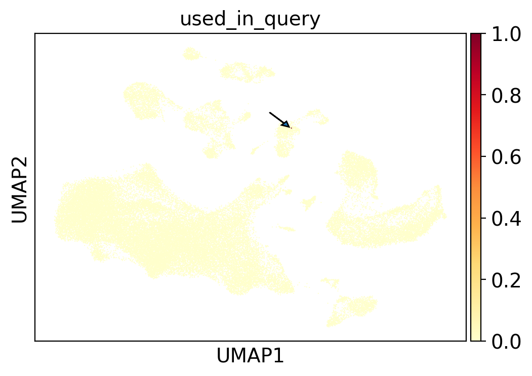
Searching for IPF-derived myofibroblasts across 23.4M cells#
This tutorial is to familiarize users with SCimilarity’s basic cell search functionality.
System requirements:
At least 64GB of RAM
0. Required software and data#
Things you need for this demo:
SCimilarity package should already be installed.
SCimilarity trained model. Download SCimilarity models. Note, this is a large tarball - downloading and uncompressing can take a several minutes.
Query data. We will use Adams et al., 2020 healthy and IPF lung scRNA-seq data. Download tutorial data.
If the model hasn’t been downloaded please uncomment and run the two command below:
[1]:
# curl -L -o /models/model_v1.1.tar.gz \
#   https://zenodo.org/records/10685499/files/model_v1.1.tar.gz?download=1
# !tar -xzvf /models/model_v1.1.tar.gz
If the data hasn’t been downloaded please uncomment and run the two command below:
[2]:
# !curl -L -o '/data/GSE136831_subsample.h5ad' \
#   https://zenodo.org/records/13685881/files/GSE136831_subsample.h5ad?download=1
[3]:
import scanpy as sc
from matplotlib import pyplot as plt

sc.set_figure_params(dpi=100)
plt.rcParams["figure.figsize"] = [6, 4]

import warnings

warnings.filterwarnings("ignore")
1. Prepare for SCimilarity: Import and normalize data#
[4]:
from scimilarity.utils import lognorm_counts, align_dataset
from scimilarity import CellQuery
Import SCimilarity - Cell query object#
[5]:
# Instantiate the CellQuery object
# Set model_path to the location of the uncompressed model
model_path = "/models/model_v1.1"
cq = CellQuery(model_path)
Load scRNA-seq data#
[6]:
# Load the tutorial data
# Set data_path to the location of the tutorial dataset
data_path = "/data/GSE136831_subsample.h5ad"
adams = sc.read(data_path)
SCimilarity pre-processing#
SCimilarity requires new data to be processed in a specific way that matches how the model was trained.
Match feature space with SCimilarity models#
SCimilarity’s gene expression ordering is fixed. New data should be reorderd to match that, so that it is consistent with how the model was trained. Genes that are not present in the new data will be zero filled to comply to the expected structure. Genes that are not present in SCimilarity’s gene ordering will be filtered out.
Note, SCimilarity was trained with high data dropout to increase robustness to differences in gene lists.
[7]:
adams = align_dataset(adams, cq.gene_order)
Normalize data consistent with SCimilarity#
It is important to match Scimilarity’s normalization so that the data matches the lognorm tp10k procedure used during model training.
[8]:
adams = lognorm_counts(adams)
With these simple steps, the data is now ready for SCimilarity. We are able to filter cells whenever we want (even after embedding) because SCimilarity handles each cell independently and can skip highly variable gene selection altogether.
2. Compute embeddings#
Using the already trained models, SCimilarity can embed your new dataset.
[9]:
adams.obsm["X_scimilarity"] = cq.get_embeddings(adams.X)
Compute visualization of embeddings#
[10]:
sc.pp.neighbors(adams, use_rep="X_scimilarity")
sc.tl.umap(adams)
3. Perform cell search#
Search for 10,000 most simliar cells across 22.7M cell reference and extract metadata for each cell.
For sub-second searches, with less frills, use cq.get_nearest_neighbors.
Note, many of the search results will be from the Adams et al. dataset, since the most similar cells will come from the same sample or study.
Input for cq.search_nearest()
Model embedding which we calculate from
cq.get_embeddings()as we did above.krepresenting the number of neighbours we would like to find.
Output of cq.search_nearest()
nn_idxs: indices of neighbour cells in the SCimilarity reference.nn_dists: the distance between neighbour cells and the query.metadata: a dataframe containing the metadata associated with each cell.
[15]:
query_cell = subsample[subsample.obs.index == "123942"]
query_embedding = query_cell.obsm["X_scimilarity"]
[16]:
%%time
k = 10000
nn_idxs, nn_dists, results_metadata = cq.search_nearest(query_embedding, k=k)
CPU times: user 7.44 s, sys: 1.88 s, total: 9.32 s
Wall time: 9.32 s
Interpret results#
Now that the query has returned the most similar cells, we can look at the cells to see which studies and conditions they are present in.
[17]:
def calculate_disease_proportions(metadata):
    study_proportions = metadata.disease.value_counts()
    return 100 * study_proportions / study_proportions.sum()


def plot_proportions(df, title=None):
    ax = df.plot(
        kind="barh", xlabel="percent of cells", title=title, grid=False, figsize=(8, 5)
    )
    ax.tick_params(axis="y", labelsize=8)
    ax.set_xticklabels([f"{int(tick)}%" for tick in ax.get_xticks()])
    plt.tight_layout()
Exclude self-referencing results#
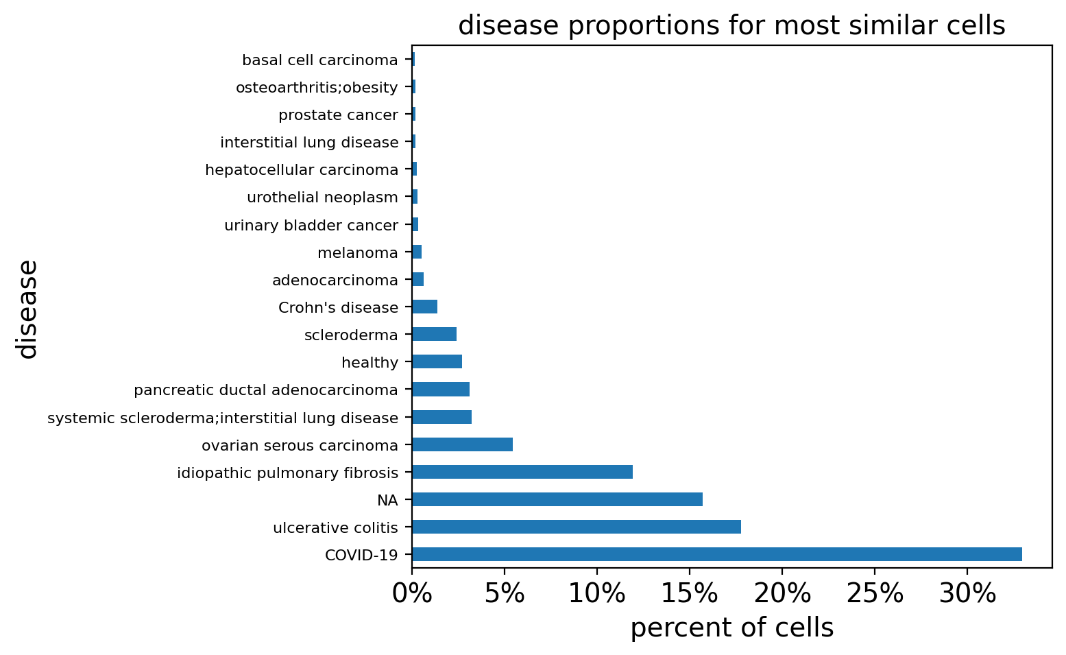
Naturally, queries searching for similar cells will highlight cells from the same study. To get a clearer view of the results, we often exclude self-referencing hits.
[18]:
query_study = "DS000011735"
filtered_result_metadata = results_metadata[results_metadata.study != query_study]
query_disease_frequencies = calculate_disease_proportions(filtered_result_metadata)
query_disease_frequencies = query_disease_frequencies[query_disease_frequencies > 0.1]
plot_proportions(
    query_disease_frequencies, title="disease proportions for most similar cells"
)
[19]:
query_disease_frequencies
[19]:
disease
COVID-19                                          32.958092
ulcerative colitis                                17.766384
NA                                                15.693268
idiopathic pulmonary fibrosis                     11.937138
ovarian serous carcinoma                           5.461436
systemic scleroderma;interstitial lung disease     3.232278
pancreatic ductal adenocarcinoma                   3.098529
healthy                                            2.697280
scleroderma                                        2.418636
Crohn's disease                                    1.359786
adenocarcinoma                                     0.646456
melanoma                                           0.534998
urinary bladder cancer                             0.334374
urothelial neoplasm                                0.312082
hepatocellular carcinoma                           0.256353
interstitial lung disease                          0.200624
prostate cancer                                    0.200624
osteoarthritis;obesity                             0.178333
basal cell carcinoma                               0.133749
Name: count, dtype: float64
This query shows higher proportion of cells in multiple diseases including COVID-19, ulcerative colitis, ILDs, and cancers compared to healthy samples. However results can be skewed by the imbalanced abundances of diseases and tissues in the query reference. We can look at how enriched these cells are by counting the number of predicted myofibroblasts (already precompted in cq.cell_metadata) across diseases for both our query hits and the full reference.
Get reference cell metadata#
Sample metadata has been curated to be able to see tissue, disease, etc for each cell. In this metadata table each row corresponds to a cell that is matched by index across the full kNN index and precomputed cell embeddings.
[20]:
ref_metadata = cq.cell_metadata
Compare to background of myofibroblasts across diseases#
To see how enriched our results are for a disease of interest, we can visualize this imbalance.
Subset the full reference metadata to cells that are predicted to be myofibroblasts.
Tabulate the cell counts by disease state.
Visualize the proportion of myofibroblasts within the reference collection in different diseases.
[21]:
myofib_meta = ref_metadata[ref_metadata.prediction.isin(["myofibroblast cell"])]
query_disease_frequencies = calculate_disease_proportions(myofib_meta)
plot_proportions(
    query_disease_frequencies[:15],
    title="disease proportions for reference myofibroblasts",
)
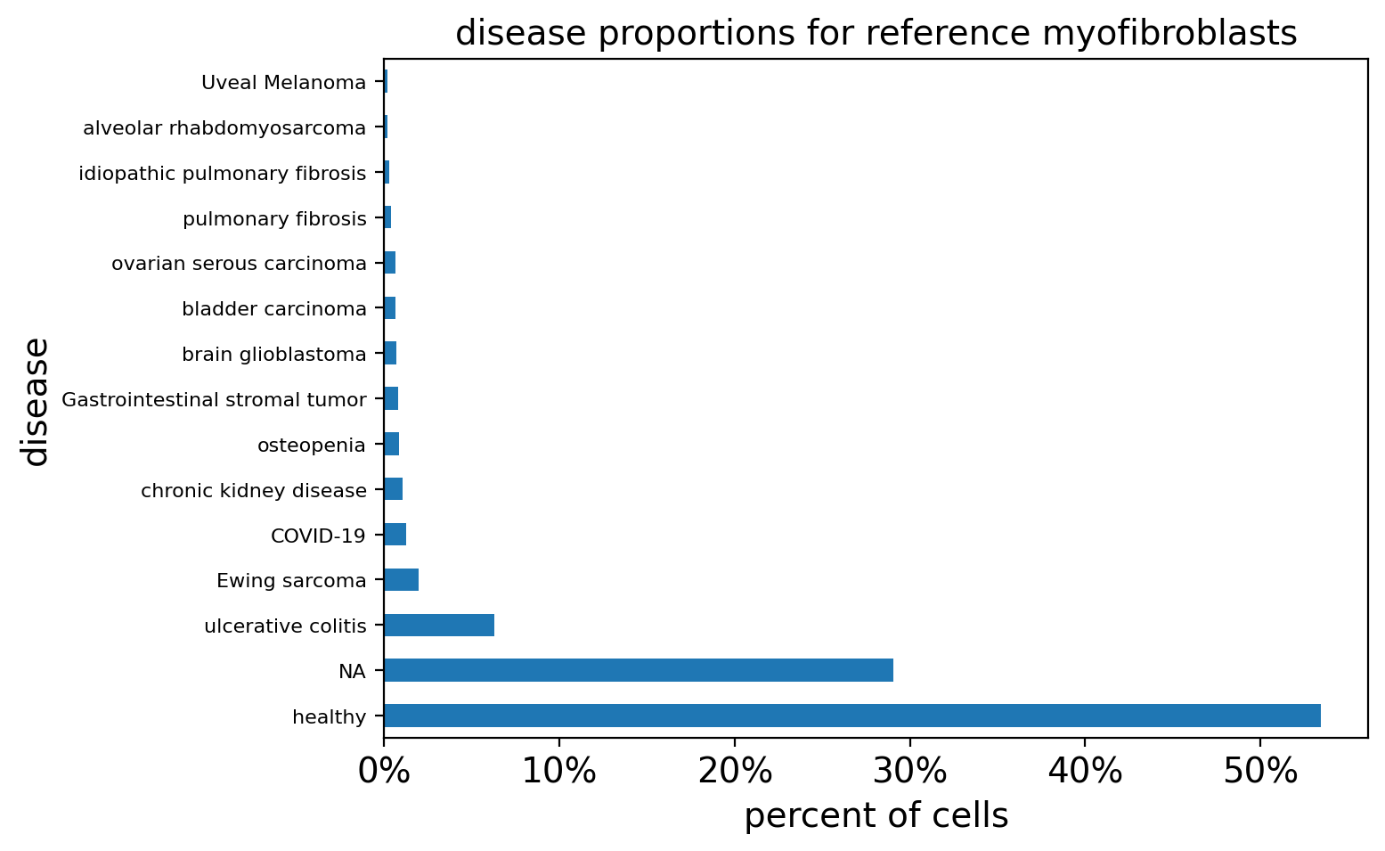
Over 50% of the myofibroblasts in the reference are from healthy tissues, while in our query they make up less than 5% of the cells most similar to our query. This confirms that these cells are in fact found in multiple conditions as highlighted earlier while they are more rare in healthy samples.
Conclusion#
This notebook outlines the basics of how to take a dataset, select a query cell, perform a cell search across our precomputed reference of 23.4M cells and summarize the results. You can use this as a template to expore cell states in other datasets you are interested in.
Keep in mind that the datasets that you analyze with SCimilarity should fit the following criteria:
Data generated from the 10x Genomics Chromium platform (models are trained using this data only).
Human scRNA-seq data.
Counts normalized with SCimilarity functions or using the same process. Different normalizations will have poor results.
Next: Advanced cell search using centroids#
This notebook demonstrated the basic cell search principle using SCimilarity. However, a single cell’s expression data is noisy and the query results from which can be highly variable even from identical cell types. This variability can be mitigated by searching using the centroid of many cells.
No matter if you search from a cell or a centroid, users must take caution to input a meaningful gene expression profile into SCimilarity’s query.
Check out the next tutorial to learn how to search cell centroids using SCimilarity!
