Fine-tune Enformer to perform binary classification on human snATAC-seq data#

In this tutorial, we learn how to fine-tune the Enformer model (https://www.nature.com/articles/s41592-021-01252-x) on the CATLAS single-nucleus ATAC-seq dataset from human tissues (http://catlas.org/humanenhancer/).

We will perform binary classification, in which the model learns to predict the probability that a given sequence is accessible in the different cell types of the dataset. For an example of regression modeling, see the next tutorial.

import anndata
import os
import importlib
import pandas as pd
import numpy as np

%matplotlib inline

Set experiment parameters#

experiment='tutorial_2'
if not os.path.exists(experiment):
    os.makedirs(experiment)

Download data#

We download the CATlas ATAC-seq binary cell type x peak matrix from the gReLU model zoo. The original source of this data is https://decoder-genetics.wustl.edu/catlasv1/humanenhancer/data/cCRE_by_cell_type/. For more details, see https://decoder-genetics.wustl.edu/catlasv1/catlas_humanenhancer/#!/.

import grelu.resources
dataset_path = grelu.resources.download_dataset(repo_id="Genentech/tutorial-2-data")

Load data#

The download_dataset function returns the path to the downloaded h5ad file containing the binarized chromatin accessibility data for multiple human cell types. We now load this as an anndata object.

ad = anndata.read_h5ad(dataset_path)
ad

AnnData object with n_obs × n_vars = 222 × 1154611
    obs: 'cell type'
    var: 'chrom', 'start', 'end', 'Class'

This contains a binary matrix representing the accessibility of 1154611 CREs measured in 222 cell types. Let us look at the components of this object:

ad.var.head()

	chrom	start	end	Class
0	chr1	9955	10355	Promoter Proximal
1	chr1	29163	29563	Promoter
2	chr1	79215	79615	Distal
3	chr1	102755	103155	Distal
4	chr1	115530	115930	Distal

ad.obs.head()

	cell type
cell type
Follicular	Follicular
Fibro General	Fibro General
Acinar	Acinar
T Lymphocyte 1 (CD8+)	T Lymphocyte 1 (CD8+)
T lymphocyte 2 (CD4+)	T lymphocyte 2 (CD4+)

The contents of this anndata object are binary values (0 or 1). 1 indicates accessibility of the peak in the cell type.

ad.X[:5, :5].todense()

matrix([[1., 0., 0., 0., 0.],
        [1., 0., 0., 0., 0.],
        [1., 0., 0., 0., 0.],
        [1., 0., 0., 0., 0.],
        [1., 0., 0., 0., 0.]], dtype=float32)

Filter peaks#

We will perform filtering of this dataset using the grelu.data.preprocess module.

First, we filter peaks within autosomes (chromosomes 1-22) or chromsomes X/Y. You can also supply autosomes or autosomesX to further restrict the chromosomes.

import grelu.data.preprocess

ad = grelu.data.preprocess.filter_chromosomes(ad, 'autosomesXY')

Keeping 1154464 intervals

Next, we drop peaks overlapping with the ENCODE blacklist regions for the hg38 genome.

ad = grelu.data.preprocess.filter_blacklist(ad, genome='hg38')

Keeping 1149915 intervals

Visualize data#

Next, we can plot the distribution of the data in various ways.

import grelu.visualize
%matplotlib inline

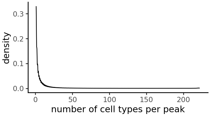
In how many accessible cell types is each peak accessible?

cell_types_per_peak = np.array(np.sum(ad.X > 0, axis=0))

grelu.visualize.plot_distribution(
    cell_types_per_peak,
    title='number of cell types per peak',
    method='density', # Alternative: histogram
    figsize=(3.6, 2), # width, height
)

../_images/01e0c8396386d57c27d2d7b89a4dc9dbc16447ac4683268ad6cada187c822a85.png

How many peaks are accessible in each cell type?

fraction_accessible_per_cell_type = np.array(np.mean(ad.X > 0, axis=1))

grelu.visualize.plot_distribution(
    fraction_accessible_per_cell_type,
    title='Fraction of peaks accessible per cell type',
    method='histogram', # alternative: density
    binwidth=0.005,
    figsize=(3.6, 2), # width, height
)

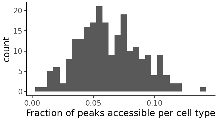
../_images/eff90699bf4257a20cff30bab130bb323b03648d4018a9b2907379a6f319e3c9.png

It seems that some cell types have very few accessible peaks. We will drop these cell types from the dataset.

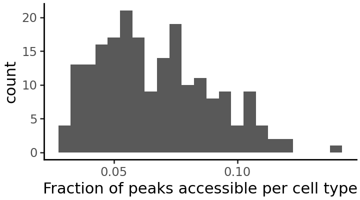
print(ad.shape)
ad = ad[ad.X.mean(axis=1) > .03, :]
print(ad.shape)

(222, 1149915)
(203, 1149915)

We can plot the distribution once again to see the effect of this filtering:

fraction_accessible_per_cell_type = np.array(np.mean(ad.X > 0, axis=1))

grelu.visualize.plot_distribution(
    fraction_accessible_per_cell_type,
    title='Fraction of peaks accessible per cell type',
    method='histogram', # alternative: density
    binwidth=0.005,
    figsize=(3.6, 2), # width, height
)

../_images/32caa9acf3f9d0fc50dc14f2a846ddeb9634b7778e696a912e101713f8fce9bd.png

Resize peaks#

Finally, since the ATAC-seq peaks can have different lengths, we resize all of them to a constant length in order to train the model. Here, we take 200 bp. We can use the resize function in grelu.sequence.utils, which contains functions to manipulate DNA sequences.

import grelu.sequence.utils
seq_len = 200

ad.var = grelu.sequence.utils.resize(ad.var, seq_len)
ad.var.head(3)

	chrom	start	end	Class
27	chr1	794997	795197	Distal
28	chr1	804833	805033	Promoter Proximal
29	chr1	816263	816463	Promoter Proximal

Split data#

We will split the peaks by chromosome to create separate sets for training, validation and testing.

train_chroms='autosomes'
val_chroms=['chr10']
test_chroms=['chr11']

ad_train, ad_val, ad_test = grelu.data.preprocess.split(
    ad,
    train_chroms=train_chroms, val_chroms=val_chroms, test_chroms=test_chroms,
)

Selecting training samples
Keeping 1004076 intervals


Selecting validation samples
Keeping 56911 intervals


Selecting test samples
Keeping 56366 intervals
Final sizes: train: (203, 1004076), val: (203, 56911), test: (203, 56366)

Make labeled sequence datasets#

grelu.data.dataset contains PyTorch Dataset classes that can load and process genomic data for training a deep learning model. Here, we use the AnnDataSeqDataset class which loads data from an AnnData object. Other available dataset classes include DFSeqDataset and BigWigSeqDataset.

We first make the training dataset. To increase model robustness we use several forms of data augmentation here: rc=True (reverse complementing the input sequence), and max_seq_shift=1 (shifting the coordinates of the input sequence by upto 1 bp in either direction; also known as jitter). We use augmentation_mode="random" which means that at each iteration, the model sees a randomly selected augmented version for each sequence.

import grelu.data.dataset

train_dataset = grelu.data.dataset.AnnDataSeqDataset(
    ad_train.copy(),
    genome='hg38',
    rc=True, # reverse complement
    max_seq_shift=1, # Shift the sequence
    augment_mode="random", # Randomly select which augmentations to apply
)

We do not apply any augmentations to the validation and test datasets (although it is possible to do so).

val_dataset = grelu.data.dataset.AnnDataSeqDataset(ad_val.copy(), genome='hg38')
test_dataset = grelu.data.dataset.AnnDataSeqDataset(ad_test.copy(), genome='hg38')

Build the enformer model#

gReLU contains many model architectures. One of these is a class called EnformerPretrainedModel. This class creates a model identical to the published Enformer model and initialized with the trained weights, but where you can change the number of transformer layers and the output head.

Models are created using the grelu.lightning module. In order to instantiate a model, we need to specify model_params (parameters for the model architecture) and train_params (parameters for training).

model_params = {
    'model_type':'EnformerPretrainedModel', # Type of model
    'n_tasks': ad.shape[0], # Number of cell types to predict
    'crop_len':0, # No cropping of the model output
    'n_transformers': 1, # Number of transformer layers; the published Enformer model has 11
}

train_params = {
    'task':'binary', # binary classification
    'lr':1e-4, # learning rate
    'logger': 'csv', # Logs will be written to a CSV file
    'batch_size': 1024,
    'num_workers': 8,
    'devices': 0, # GPU index
    'save_dir': experiment,
    'optimizer': 'adam',
    'max_epochs': 10,
    'checkpoint': True, # Save checkpoints
}

import grelu.lightning
model = grelu.lightning.LightningModel(model_params=model_params, train_params=train_params)

Train the model#

We train the model on the new training dataset using the train_on_dataset method. Note that here, we update the weights of the entire model during training. If you want to hold the enformer weights fixed and only learn a linear layer from the enformer embedding to the outputs, see the tune_on_dataset method.

# See the 'tutorial_2' folder for logs
trainer = model.train_on_dataset(
    train_dataset=train_dataset,
    val_dataset=val_dataset,
)

/gpfs/scratchfs01/site/u/lala8/conda/envs/grelu-test/lib/python3.10/site-packages/rich/live.py:260: UserWarning: 
install "ipywidgets" for Jupyter support

┏━━━━━━━━━━━━━━━━━━━━━━━━━━━┳━━━━━━━━━━━━━━━━━━━━━━━━━━━┓
┃      Validate metric      ┃       DataLoader 0        ┃
┡━━━━━━━━━━━━━━━━━━━━━━━━━━━╇━━━━━━━━━━━━━━━━━━━━━━━━━━━┩
│       val_accuracy        │    0.49347996711730957    │
│         val_auroc         │    0.49767163395881653    │
│        val_avgprec        │    0.10673108696937561    │
│        val_best_f1        │    0.17083537578582764    │
│         val_loss          │    0.6943522095680237     │
└───────────────────────────┴───────────────────────────┘

┏━━━┳━━━━━━━━━━━━━━┳━━━━━━━━━━━━━━━━━━━━━━━━━┳━━━━━━━━┳━━━━━━━┳━━━━━━━┓
┃   ┃ Name         ┃ Type                    ┃ Params ┃ Mode  ┃ FLOPs ┃
┡━━━╇━━━━━━━━━━━━━━╇━━━━━━━━━━━━━━━━━━━━━━━━━╇━━━━━━━━╇━━━━━━━╇━━━━━━━┩
│ 0 │ model        │ EnformerPretrainedModel │ 72.1 M │ train │     0 │
│ 1 │ loss         │ BCEWithLogitsLoss       │      0 │ train │     0 │
│ 2 │ val_metrics  │ MetricCollection        │      0 │ train │     0 │
│ 3 │ test_metrics │ MetricCollection        │      0 │ train │     0 │
│ 4 │ transform    │ Identity                │      0 │ train │     0 │
└───┴──────────────┴─────────────────────────┴────────┴───────┴───────┘

Trainable params: 72.1 M                                                                                           
Non-trainable params: 0                                                                                            
Total params: 72.1 M                                                                                               
Total estimated model params size (MB): 288                                                                        
Modules in train mode: 240                                                                                         
Modules in eval mode: 0                                                                                            
Total FLOPs: 0

/gpfs/scratchfs01/site/u/lala8/conda/envs/grelu-test/lib/python3.10/site-packages/rich/live.py:260: UserWarning: 
install "ipywidgets" for Jupyter support

/gpfs/scratchfs01/site/u/lala8/conda/envs/grelu-test/lib/python3.10/site-packages/rich/live.py:260: UserWarning: 
install "ipywidgets" for Jupyter support

Load best model from checkpoint#

During training, the performance of the model on the validation set is checked after each epoch. We will load the version of the model that had the best validation set performance.

best_checkpoint = trainer.checkpoint_callback.best_model_path
print(best_checkpoint)
model = grelu.lightning.LightningModel.load_from_checkpoint(best_checkpoint)

tutorial_2/2026_03_03_15_54/version_0/checkpoints/epoch=7-step=7848.ckpt

Calculate performance metrics on the test set#

We calculate global performance metrics using the test_on_dataset method.

test_metrics = model.test_on_dataset(
    test_dataset,
    devices=0,
    num_workers=8,
    batch_size=1024,
)

┏━━━━━━━━━━━━━━━━━━━━━━━━━━━┳━━━━━━━━━━━━━━━━━━━━━━━━━━━┓
┃        Test metric        ┃       DataLoader 0        ┃
┡━━━━━━━━━━━━━━━━━━━━━━━━━━━╇━━━━━━━━━━━━━━━━━━━━━━━━━━━┩
│       test_accuracy       │    0.9458667039871216     │
│        test_auroc         │    0.9044811725616455     │
│       test_avgprec        │    0.6075653433799744     │
│       test_best_f1        │    0.5681172013282776     │
│         test_loss         │    0.15379782021045685    │
└───────────────────────────┴───────────────────────────┘

test_metrics is a dataframe containing metrics for each model task.

test_metrics.head()

	test_accuracy	test_auroc	test_avgprec	test_best_f1
Follicular	0.909236	0.878971	0.628441	0.578610
Fibro General	0.916510	0.883105	0.625623	0.575389
Acinar	0.944186	0.913036	0.650671	0.602352
T Lymphocyte 1 (CD8+)	0.962034	0.930548	0.635034	0.589981
T lymphocyte 2 (CD4+)	0.967108	0.939110	0.618744	0.573214

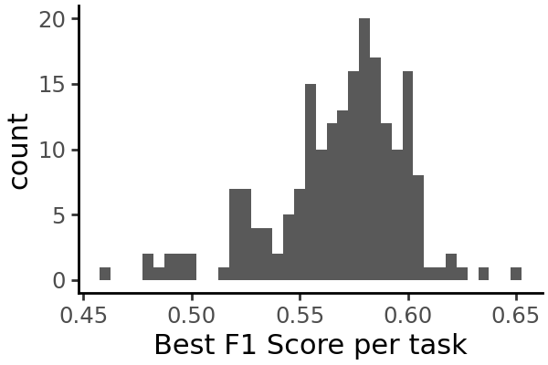
Visualize performance metrics#

We can plot the distribution of each metric across all cell types:

grelu.visualize.plot_distribution(
    test_metrics.test_best_f1,
    method='histogram',
    title='Best F1 Score per task',
    binwidth=0.005,
    figsize=(3,2),
)

../_images/60b3ee2a3f59f9df4c48124926e39d06323b8a533127ca43cee13ff91b4cdc1f.png

grelu.visualize.plot_distribution(
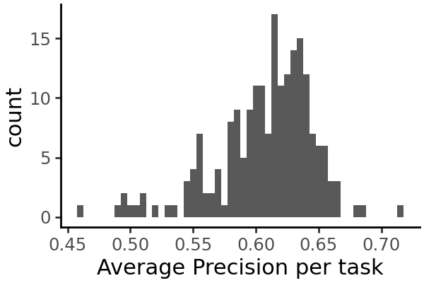
    test_metrics.test_avgprec,
    method='histogram',
    title='Average Precision per task',
    binwidth=0.005,
    figsize=(3,2),
)

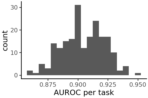
../_images/6edefe433ecb13faf99c2cf205f588f5bc141668f5cd39b454d726667a69fee5.png

grelu.visualize.plot_distribution(
    test_metrics.test_auroc,
    method='histogram',
    title='AUROC per task',
    binwidth=0.005,
    figsize=(3,2),
)

../_images/d474d876c7dd9249c121436f69e677a1b194ea52541994de9bb85790aeac9856.png

Run inference on the test set#

Instead of overall metrics, we can also get the individual predictions for each test set example.

probs = model.predict_on_dataset(
    test_dataset,
    devices=0,
    num_workers=8,
    batch_size=1024,
    return_df=True # Return the output as a pandas dataframe
)

probs.head()

	Follicular	Fibro General	Acinar	T Lymphocyte 1 (CD8+)	T lymphocyte 2 (CD4+)	Natural Killer T	Naive T	Fibro Epithelial	Cardiac Pericyte 1	Pericyte General 1	...	Fetal Cardiac Fibroblast	Fetal Fibro General 2	Fetal Fibro Muscle 1	Fetal Fibro General 3	Fetal Mesangial 2	Fetal Stellate	Fetal Alveolar Epithelial 1	Fetal Cilliated	Fetal Excitatory Neuron 1	Fetal Excitatory Neuron 2
0	0.037320	0.059341	0.019623	0.057960	0.022940	0.037132	0.024256	0.060020	0.036380	0.044111	...	0.096488	0.084068	0.098517	0.111082	0.123722	0.055901	0.168764	0.117609	0.134788	0.044917
1	0.045293	0.040371	0.026782	0.025121	0.012357	0.010523	0.011736	0.027949	0.032551	0.026512	...	0.084573	0.056361	0.049276	0.085011	0.076023	0.030324	0.179506	0.081972	0.063167	0.018129
2	0.076708	0.127368	0.057874	0.060736	0.036988	0.032808	0.036318	0.105995	0.112944	0.101309	...	0.183218	0.162204	0.136362	0.171209	0.238024	0.089201	0.274355	0.169164	0.204561	0.066065
3	0.071490	0.027930	0.013738	0.020133	0.012074	0.013508	0.009373	0.023522	0.023282	0.020539	...	0.033375	0.021606	0.019337	0.032877	0.030444	0.012405	0.072734	0.055420	0.034482	0.014244
4	0.012588	0.018428	0.010383	0.121269	0.102168	0.110026	0.067189	0.007175	0.014089	0.004672	...	0.009173	0.005470	0.005460	0.012376	0.007533	0.003261	0.038494	0.018055	0.011567	0.006286

5 rows × 203 columns

Since this is a binary classification model, the output takes the form of probabilities ranging from 0 to 1. We interpret these as the predicted probabilities of the element being accessible in each cell type.

Plot additional visualizations of the test set predictions#

We can plot a calibration curve for all the tasks. This shows us the fraction of true positive examples, for different levels of model-predicted probability.

grelu.visualize.plot_calibration_curve(
    probs, labels=test_dataset.labels, aggregate=False, show_legend=False
)

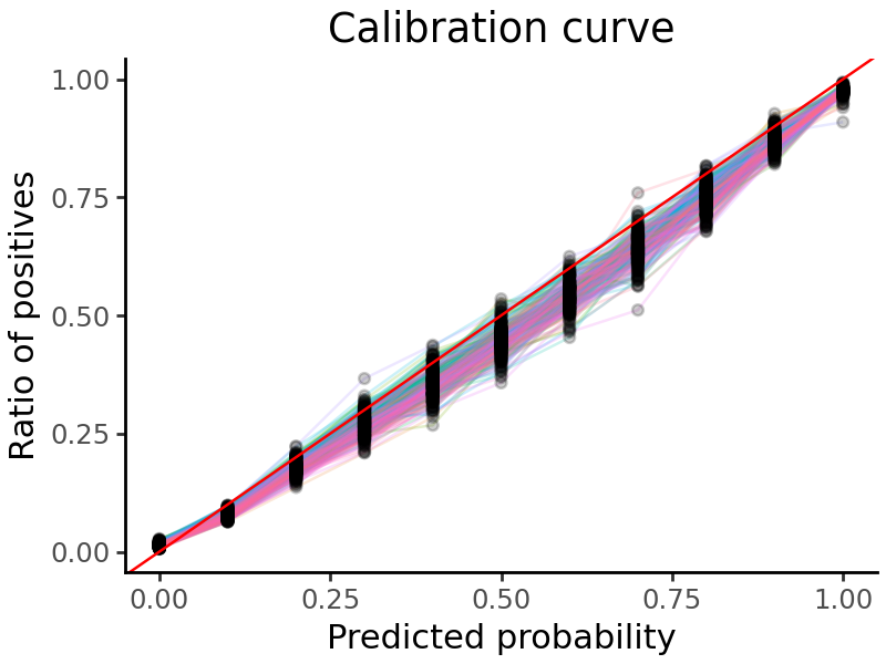
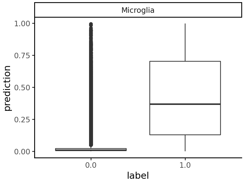
../_images/96c780e90f344cc963fe8b2969b062fb330662803a04faf2aee885181622e675.png

We can also pick any cell type and compare the predictions on accessible and non-accessible elements.

grelu.visualize.plot_binary_preds(
    probs,
    labels=test_dataset.labels,
    tasks='Microglia',
    figure_size=(3, 2) # Width, height
)

../_images/a6c4de85fab778e2d86f49f6a7b4381ebf1420a07d56119e7ed38a564315941d.png

Interpret model predictions (for microglia) using TF-modisco#

Suppose we want to focus specifically on Microglia. We can create a transform - a class that takes in the model’s prediction and returns a function of the prediction, e.g. the prediction for only a subset of cell types that we are interested in. Then, all subsquent analyses that we do will be based only on this subset of the full prediction matrix.

Transforms can also compute more complicated functions of the model’s output - for example, the Specificity class of transforms take in the full set of predictions produced by the model and compute the predicted specificity of each sequence to a particular cell type or otuput track.

In this example, we use the Specificity transform to analyze the predicted cell type specificity of sequences in microglia - i.e. the predicted accessibility in microglia minus the mean predicted accessibility in other cell types. See the Aggregate class if you want to just subset the predictions to microglia.

from grelu.transforms.prediction_transforms import Specificity

microglia_scorer = Specificity(
    on_tasks = ["Microglia"],
    model = model,
    compare_func='subtract' # Subtract the prediction in other cell types from the prediction in microglia
)

The simplest way to use a transform is to apply it directly to the model’s predictions using the .compute() method. Here, we apply this microglia specificity transform to the test set predictions:

# Transforms expect a 3-D input - add an axis 2 to the predictions.
mcg_specificity = microglia_scorer.compute(np.expand_dims(probs, 2)).squeeze()

# This is the predicted specificity for each test sequence in microglia
mcg_specificity[:5]

array([-0.02669976, -0.0286902 , -0.06530956, -0.01327392,  0.03015377],
      dtype=float32)

We can now select the 250 test set peaks with the highest predicted specificity in microglia:

mcg_peaks = ad.var.iloc[np.argsort(mcg_specificity)].tail(250)
mcg_peaks

	chrom	start	end	Class
48604	chr1	110228431	110228631	Distal
9045	chr1	17426393	17426593	Distal
56231	chr1	153465814	153466014	Distal
22304	chr1	43446480	43446680	Promoter Proximal
17265	chr1	32701425	32701625	Promoter Proximal
...	...	...	...	...
54009	chr1	146987608	146987808	Distal
18729	chr1	36233365	36233565	Distal
52592	chr1	118552721	118552921	Distal
12489	chr1	23645409	23645609	Distal
22411	chr1	43595659	43595859	Distal

250 rows × 4 columns

But transforms are more powerful than this - they allow you to do any downstream task, e.g. interpretation, variant effect prediction and design, with respect to the computed quantity.

Here, we will run TF-Modisco on these selected peaks. TF-Modisco identifies motifs that consistently contribute to the model’s output. Since we are using the microglia_scorer filter to compute predicted specificity to microglia, we will only get motifs that contribute to increased or decreased specificity. We also use TOMTOM to match the TF-Modisco motifs to a set of reference motifs. Here, we use the HOCOMOCO v12 motif set (https://hocomoco12.autosome.org/).

See the subsequent tutorials for more examples of how to use transforms.

%%time
import grelu.interpret.modisco
grelu.interpret.modisco.run_modisco(
    model,
    seqs=mcg_peaks, 
    genome="hg38",
    prediction_transform=microglia_scorer, # Attributions will be calculated with respect to this output
    meme_file="hocomoco_v13", # We will compare the Modisco CWMs to HOCOMOCO motifs
    method="saliency", # Base-level attribution scores will be calculated using saliency. You can also use ISM here.
    correct_grad=True, # Gradient correction; only applied with saliency
    out_dir=experiment,
    batch_size=256,
    devices=0,
    num_workers=32,
    seed=0,

    # Here, we are demonstrating this function on a small number of peaks,
    # So we set these modisco parameters to a low value. In real runs, we suggest
    # using larger or default values.
    min_metacluster_size=6,
    final_min_cluster_size=6,    
)

Getting attributions
Running modisco
4 positive and 5 negative patterns were found.
Writing modisco output
Creating sequence logos
Creating html report
Running TOMTOM
CPU times: user 1min 46s, sys: 1.74 s, total: 1min 47s
Wall time: 1min 24s

Load TOMTOM output for modisco motifs#

The full output of TF-Modisco and TOMTOM can be found in the experiment folder. Here, we read the output of TOMTOM and list the significant TOMTOM matches, i.e. known TF motifs that are similar to those found by TF-MoDISco.

tomtom_file = os.path.join(experiment, 'tomtom.csv')
tomtom = pd.read_csv(tomtom_file, index_col=0)

tomtom[tomtom['q-value'] < 0.001] # Display most significant matches

	Query_ID	Target_ID	Optimal_offset	p-value	E-value	q-value	Overlap	Query_consensus	Target_consensus	Orientation
175	pos_pattern_0	EHF.H13CORE.0.P.B	2.0	8.607895e-08	0.000139	0.000195	13.0	CACTTCCTCCTTG	GAACCAGGAAGTGGG	-
182	pos_pattern_0	ELF4.H13CORE.1.M.B	1.0	1.090203e-06	0.001756	0.000930	13.0	CACTTCCTCCTTG	GGAAACAGGAAGTAA	-
183	pos_pattern_0	ELF5.H13CORE.0.PSM.A	1.0	5.438433e-08	0.000088	0.000195	13.0	CACTTCCTCCTTG	AGGAAGGAGGAAGTAA	-
192	pos_pattern_0	ERF.H13CORE.0.PS.A	0.0	1.100122e-07	0.000177	0.000195	11.0	CACTTCCTCCTTG	AACAGGAAGTG	-
207	pos_pattern_0	ETS2.H13CORE.1.P.B	1.0	7.843389e-07	0.001264	0.000758	11.0	CACTTCCTCCTTG	GACCGGAAGTGG	-
218	pos_pattern_0	ETV6.H13CORE.1.P.B	1.0	8.021184e-09	0.000013	0.000058	11.0	CACTTCCTCCTTG	AAGAGGAAGTGG	-
997	pos_pattern_0	SPI1.H13CORE.0.P.B	1.0	4.753351e-09	0.000008	0.000058	13.0	CACTTCCTCCTTG	AAAAGAGGAAGTGA	-
998	pos_pattern_0	SPI1.H13CORE.1.S.B	1.0	9.519393e-08	0.000153	0.000195	11.0	CACTTCCTCCTTG	AAGGGGAAGTAG	-
999	pos_pattern_0	SPIB.H13CORE.0.P.B	4.0	3.030316e-08	0.000049	0.000146	12.0	CACTTCCTCCTTG	AAAGAGGAAGTGAAAG	-
1001	pos_pattern_0	SPIB.H13CORE.2.SM.B	1.0	9.557814e-07	0.001540	0.000866	13.0	CACTTCCTCCTTG	GGGAATGAGGAAGTAG	-
2101	pos_pattern_1	KLF14.H13CORE.1.P.C	-14.0	7.038565e-07	0.001134	0.000729	23.0	AGGTCAACCATACGCCCACTCCCGTCACTCCCCCGAGG	GAGGGGGCGGGGCCGGGGGGGGG	-
2971	pos_pattern_1	ZN557.H13CORE.0.P.C	-2.0	6.183836e-07	0.000996	0.000690	25.0	AGGTCAACCATACGCCCACTCCCGTCACTCCCCCGAGG	GAACCTGGAAGTGGATATTTGTGGG	-
3731	pos_pattern_2	KMT2A.H13CORE.0.P.B	-6.0	1.209336e-07	0.000195	0.000195	23.0	GGCCTCACGAGGCCCAGGCGCCGCCGCGCGGGCGCCAGCGGCCCCAC	CCCCGCCGCCGCCGCCGCCGCCC	+
6474	neg_pattern_0	ATF3.H13CORE.0.P.B	0.0	3.897465e-07	0.000628	0.000514	7.0	TGAGTCA	GGATGACTCA	-
6986	neg_pattern_0	MAFA.H13CORE.1.M.C	4.0	2.608469e-07	0.000420	0.000378	7.0	TGAGTCA	AAAATTGCTGACTCAGCAA	-
6993	neg_pattern_0	MAFK.H13CORE.0.PS.A	3.0	1.169238e-06	0.001884	0.000942	7.0	TGAGTCA	AAAATTGCTGACTCAGCA	-
7076	neg_pattern_0	NF2L2.H13CORE.0.P.B	2.0	7.294213e-08	0.000118	0.000195	7.0	TGAGTCA	GCTGAGTCATGCTGA	+
11928	neg_pattern_3	NFIA.H13CORE.0.P.B	-20.0	5.547534e-07	0.000894	0.000670	8.0	ATCTGAGACTCTGGGGAAGCCTGCCAGGACCTCATCC	CTTGGCAG	-