Train a single-task regression model from scratch#
In this tutorial, we train a single-task convolutional regression model to predict total coverage over ATAC-seq peaks, starting from an ATAC-seq fragment file.
import os
import numpy as np
import pandas as pd
import torch
Set experiment parameters#
experiment='tutorial_3'
if not os.path.exists(experiment):
    os.makedirs(experiment)
Peak and fragment files#
We downloaded pseudobulk scATAC data for human microglia from Corces et al. (2020): https://www.nature.com/articles/s41588-020-00721-x. Here, we use the grelu.resources module to download the fragment file and peak file from the model zoo:
import grelu.resources
# Download these datasets into local directories

fragment_file_path = grelu.resources.download_dataset(
    repo_id="Genentech/microglia-scatac-tutorial-data", filename="fragment_file.bed")

peak_file_path = grelu.resources.download_dataset(
    repo_id="Genentech/microglia-scatac-tutorial-data", filename="peak_file.narrowPeak")
# Paths to files
frag_file = fragment_file_path
peak_file = peak_file_path
Set parameters#
seq_len=2114 # Length of the input sequence
label_len=1000 # Length over which we calculate total coverage
val_chroms=["chr10"]
test_chroms=["chr11"]
genome="hg38"
Read peak file#
We read peak coordinates from the narrowPeak file.
import grelu.io.bed

peaks = grelu.io.bed.read_narrowpeak(peak_file)
peaks.tail(3)
| chrom | start | end | name | score | strand | signal | pvalue | qvalue | summit | |
|---|---|---|---|---|---|---|---|---|---|---|
| 83316 | chrY | 56870777 | 56870983 | Microglia_full_peak_83318 | 94 | . | 3.83352 | 11.58170 | 9.41381 | 116 |
| 83317 | chrY | 56873629 | 56873811 | Microglia_full_peak_83319 | 49 | . | 3.01171 | 7.02098 | 4.99754 | 105 |
| 83318 | chrY | 56874075 | 56874225 | Microglia_full_peak_83320 | 42 | . | 2.86533 | 6.19767 | 4.20704 | 17 |
Summit-center peaks#
We extract the genomic coordinates for the 2114 bases surrounding the summit of each peak.
import grelu.data.preprocess

peaks = grelu.data.preprocess.extend_from_coord(
    peaks,
    seq_len=seq_len,
    center_col="summit"
)
peaks.tail(3)
| chrom | start | end | |
|---|---|---|---|
| 83316 | chrY | 56869836 | 56871950 |
| 83317 | chrY | 56872677 | 56874791 |
| 83318 | chrY | 56873035 | 56875149 |
Filter peaks#
We filter the peaks to include only those within autosomes. You can also use “autosomesX” or “autosomesXY” to include sex chromosomes.
peaks = grelu.data.preprocess.filter_chromosomes(peaks, 'autosomes')
Keeping 80823 intervals
We drop peaks that are close to ENCODE hg38 blacklist regions.
peaks = grelu.data.preprocess.filter_blacklist(
    peaks,
    genome=genome,
    window=50 # Remove peaks if they are within 50 bp of a blacklist region
)
Keeping 80028 intervals
Get GC matched negative regions#
To ensure that the model also learns to recognize regions that are not peaks, we will include a set of “negative” (non-peak) regions with similar GC content to the peaks.
negatives = grelu.data.preprocess.get_gc_matched_intervals(
    peaks,
    binwidth=0.02, # resolution of measuring GC content
    genome=genome,
    chroms="autosomes", # negative regions will also be chosen from autosomes
    seed=0,
)
negatives.head(3)
Extracting matching intervals
Filtering blacklist
Keeping 77148 intervals
| chrom | start | end | |
|---|---|---|---|
| 39048 | chr1 | 801206 | 803320 |
| 13936 | chr1 | 813890 | 816004 |
| 20216 | chr1 | 858284 | 860398 |
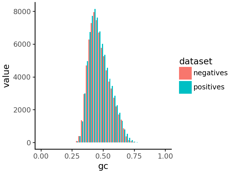
We can visualize a histogram of GC content in the peaks and negative regions to verify that they are similar.
Combine peaks and negative regions#
The full dataset includes both peaks and negative regions.
regions = pd.concat([peaks, negatives])
len(regions)
157176
Make BigWig file#
We convert the ATAC-seq fragment file into a bigWig file which contains the number of Tn5 insertions at each position. Note that this command requires bedtools and bedGraphToBigWig to be installed.
bw_file = grelu.data.preprocess.make_insertion_bigwig(
    frag_file = frag_file,
    plus_shift=0,
    minus_shift=1, # This corrects the +4/-5 Tn5 shift to a +4/-4 shift
    genome=genome,
    chroms="autosomes", # The output bigWig file contains coverage over autosomes.
)
Making bedgraph file
cat /home/lala8/.cache/huggingface/hub/datasets--Genentech--microglia-scatac-tutorial-data/snapshots/06d49b4a361b9a40e1cabf83f50030ba00a13a03/fragment_file.bed | awk -v OFS="\t" '{print $1,$2+0,$3,1000,0,"+";
    print $1,$2,$3+1,1000,0,"-"}' | sort -k1,1 | grep -e ^chr1 -e ^chr2 -e ^chr3 -e ^chr4 -e ^chr5 -e ^chr6 -e ^chr7 -e ^chr8 -e ^chr9 -e ^chr10 -e ^chr11 -e ^chr12 -e ^chr13 -e ^chr14 -e ^chr15 -e ^chr16 -e ^chr17 -e ^chr18 -e ^chr19 -e ^chr20 -e ^chr21 -e ^chr22  | bedtools genomecov -bg -5 -i stdin -g /home/lala8/.local/share/genomes/hg38/hg38.fa.sizes | bedtools sort -i stdin > ./fragment_file.bedGraph
Making bigWig file
bedGraphToBigWig ./fragment_file.bedGraph /home/lala8/.local/share/genomes/hg38/hg38.fa.sizes ./fragment_file.bw
Deleting temporary files
Split data by chromosome#
We now split the dataset by chromosome to create separate datasets for training, validation and testing.
train, val, test = grelu.data.preprocess.split(
    regions, val_chroms=val_chroms, test_chroms=test_chroms)
Selecting training samples
Keeping 140654 intervals


Selecting validation samples
Keeping 8115 intervals


Selecting test samples
Keeping 8407 intervals
Final sizes: train: (126394, 3), val: (699, 3), test: (791, 3)
Make labeled datasets#
We now make pytorch dataset objects in order to load paired sequences and coverage values from the genome and the bigWig file. We use the BigWigSeqDataset class.
We first make the training dataset. To increase model robustness we use several forms of data augmentation here: rc=True (reverse complementing the input sequence), max_seq_shift=2 (shifting the coordinates of the input sequence by upto 2 bp in either direction; also known as jitter), and max_pair_shift=20 (shifting both the input sequence and the region for which to calculate coverage by upto 20 bp in either direction).
Further, we use label_aggfunc="sum" which means that the label will be the summed coverage over the central region of the interval.
import grelu.data.dataset
train_ds = grelu.data.dataset.BigWigSeqDataset(
    intervals = train,
    bw_files=[bw_file],
    label_len=label_len,
    label_aggfunc="sum",
    rc=True, # reverse complement
    max_seq_shift=2, # Shift the sequence
    max_pair_shift=20, # Shift both sequence and label
    augment_mode="random",
    seed=0,
    genome=genome,
)
We do not apply any augmentations to the validation and test datasets (although it is possible to do so).
val_ds = grelu.data.dataset.BigWigSeqDataset(
    intervals = val,
    bw_files=[bw_file],
    label_len=label_len,
    label_aggfunc="sum",
    genome=genome,
)

test_ds = grelu.data.dataset.BigWigSeqDataset(
    intervals = test,
    bw_files=[bw_file],
    label_len=label_len,
    label_aggfunc="sum",
    genome=genome,
)

len(train_ds), len(val_ds), len(test_ds)
(126394, 699, 791)
Build model#
model_params = {
    'model_type':'DilatedConvModel',
    'crop_len':(seq_len-label_len)//2,
    'n_tasks':1,
    'channels':512,
    'n_conv':8,
}

train_params = {
    'task':'regression',
    'loss': 'poisson', # Poisson loss. Other regression loss functions are "mse" and "poisson_multinomial"
    'logger':'csv',
    'lr':1e-4,
    'batch_size':512,
    'max_epochs':10,
    'devices':0,
    'num_workers':16,
    'save_dir':experiment,
}

import grelu.lightning
model = grelu.lightning.LightningModel(model_params, train_params)
Train model#
# See the tutorial_3 folder for logs.
trainer = model.train_on_dataset(train_ds, val_ds)
┏━━━━━━━━━━━━━━━━━━━━━━━━━━━┳━━━━━━━━━━━━━━━━━━━━━━━━━━━┓
┃      Validate metric      ┃       DataLoader 0        ┃
┡━━━━━━━━━━━━━━━━━━━━━━━━━━━╇━━━━━━━━━━━━━━━━━━━━━━━━━━━┩
│         val_loss          │       1111.22265625       │
│          val_mse          │       228985.859375       │
│        val_pearson        │   -0.36367514729499817    │
└───────────────────────────┴───────────────────────────┘
┏━━━┳━━━━━━━━━━━━━━┳━━━━━━━━━━━━━━━━━━┳━━━━━━━━┳━━━━━━━┳━━━━━━━┓
┃   ┃ Name         ┃ Type             ┃ Params ┃ Mode  ┃ FLOPs ┃
┡━━━╇━━━━━━━━━━━━━━╇━━━━━━━━━━━━━━━━━━╇━━━━━━━━╇━━━━━━━╇━━━━━━━┩
│ 0 │ model        │ DilatedConvModel │  5.6 M │ train │     0 │
│ 1 │ loss         │ PoissonNLLLoss   │      0 │ train │     0 │
│ 2 │ val_metrics  │ MetricCollection │      0 │ train │     0 │
│ 3 │ test_metrics │ MetricCollection │      0 │ train │     0 │
│ 4 │ transform    │ Identity         │      0 │ train │     0 │
└───┴──────────────┴──────────────────┴────────┴───────┴───────┘
Trainable params: 5.6 M
Non-trainable params: 0
Total params: 5.6 M
Total estimated model params size (MB): 22
Modules in train mode: 118
Modules in eval mode: 0
Total FLOPs: 0
Load the best model version#
best_checkpoint = trainer.checkpoint_callback.best_model_path
print(best_checkpoint)
tutorial_3/2026_04_03_10_18/version_0/checkpoints/epoch=9-step=2470.ckpt
model = grelu.lightning.LightningModel.load_from_checkpoint(best_checkpoint)
Evaluate model#
We now evaluate the model’s performance on the test dataset.
test_metrics = model.test_on_dataset(
    test_ds,
    batch_size=256,
    devices=0,
    num_workers=8
)

test_metrics
┏━━━━━━━━━━━━━━━━━━━━━━━━━━━┳━━━━━━━━━━━━━━━━━━━━━━━━━━━┓
┃        Test metric        ┃       DataLoader 0        ┃
┡━━━━━━━━━━━━━━━━━━━━━━━━━━━╇━━━━━━━━━━━━━━━━━━━━━━━━━━━┩
│         test_loss         │    119.36114501953125     │
│         test_mse          │      106301.9296875       │
│       test_pearson        │     0.679975688457489     │
└───────────────────────────┴───────────────────────────┘
| test_mse | test_pearson | |
|---|---|---|
| fragment_file | 106301.929688 | 0.679976 |
Run inference on held out sequences#
We can now get the predicted total coverage for each sequence in the test set.
preds = model.predict_on_dataset(
    test_ds, devices=0, num_workers=8
    )
preds.shape
(791, 1, 1)
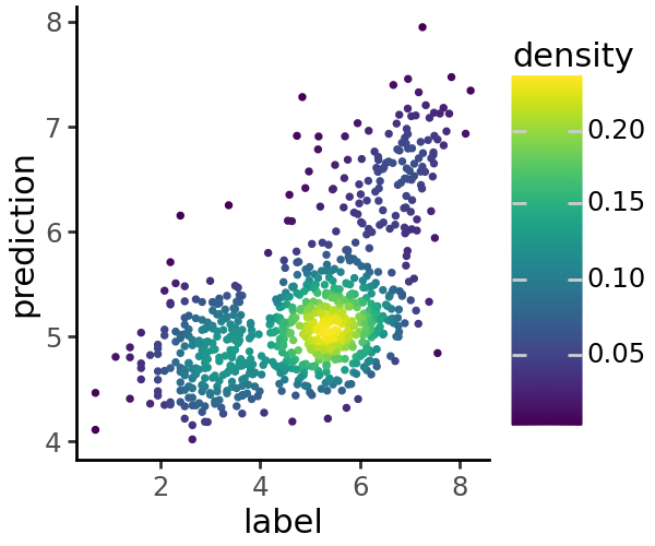
We can visualize a scatter plot of predicted vs. true coverage values

