Predict Effects of Alzheimer’s Variants Using ATAC Models

In this tutorial, we demonstrate how to predict the impact of sequence variation using a trained gReLU model.

import anndata as ad
import pandas as pd
import numpy as np
import os

Load the CATlas model

This is a binary classification model trained on snATAC-seq data from Catlas (http://catlas.org/humanenhancer/). This model predicts the probability that an input sequence will be accessible in various cell types.

import grelu.resources
model = grelu.resources.load_model(project='human-atac-catlas', model_name='model')

View the model’s metadata

model.data_params is a dictionary containing metadata about the data used to train the model. Let’s look at what information is stored:

for key in list(model.data_params.keys())[:21]:
    if key !="tasks":
        print(key, model.data_params[key])

train_bin_size 1
train_chroms ['chr18', 'chr5', 'chr1', 'chr17', 'chr9', 'chr19', 'chr8', 'chr21', 'chr14', 'chr20', 'chr22', 'chr10', 'chr15', 'chr12', 'chr16', 'chr3', 'chr4', 'chr11', 'chr2', 'chr6']
train_end both
train_genome hg38
train_label_aggfunc None
train_label_len 200
train_label_transform_func None
train_max_label_clip None
train_max_pair_shift 0
train_max_seq_shift 1
train_min_label_clip None
train_n_alleles 1
train_n_augmented 1
train_n_seqs 1022128
train_n_tasks 204
train_padded_label_len 200
train_padded_seq_len 202
train_predict False
train_rc True
train_seq_len 200

Note the parameter train_seq_len. This tells us that the model was trained on 200 bp long sequences.

model.data_params['tasks'] is a large dictionary containing metadata about the output tracks that the model predicts. We can collect these into a dataframe called tasks:

tasks = pd.DataFrame(model.data_params['tasks'])
tasks.head(3)

	name	cell type
0	Follicular	Follicular
1	Fibro General	Fibro General
2	Acinar	Acinar

Load Alzheimer’s Variants from GWAS Catalog (Jansen et al. 2019 meta-analysis)

Download a small subset of variants from the AD sumstats file from this meta-analysis study. This contains 1,000 variants mapped to the hg19 genome.

import grelu.resources

variant_dir = grelu.resources.get_artifact(
    project='alzheimers-variant-tutorial',
    name='dataset'
).download()

variant_file = os.path.join(variant_dir, "variants.txt")

variants = pd.read_table(variant_file)
variants.head(3)

	snpid	chrom	pos	alt	ref	rsid	zscore	pval	nsum	neff	direction	eaf	beta	se
0	6:32630634_G_A	chr6	32630634	G	A	6:32630634	3.974476	0.000071	71639	71639.0	?+?+	0.2237	0.025194	0.006339
1	6:32630797_A_G	chr6	32630797	A	G	6:32630797	4.040244	0.000053	71639	71639.0	?+?+	0.2435	0.024866	0.006155
2	6:32630824_T_C	chr6	32630824	T	C	6:32630824	3.921736	0.000088	71639	71639.0	?+?+	0.1859	0.026630	0.006790

Filter variants

from grelu.data.preprocess import filter_blacklist, filter_chromosomes
from grelu.variant import filter_variants

Remove indels, since we don’t support them for now. We also remove variants where one of the alleles contains Ns.

variants = filter_variants(variants, max_del_len=0, max_insert_len=0, standard_bases=True)

Initial number of variants: 1000
Final number of variants: 989

Remove non-standard chromosomes

variants = filter_chromosomes(variants, include='autosomesXY')

Keeping 989 intervals

Remove SNPs from unmappable regions

variants = filter_blacklist(variants, genome="hg19", window=100).reset_index(drop=True)

Keeping 988 intervals

variants.head(3)

	snpid	chrom	pos	alt	ref	rsid	zscore	pval	nsum	neff	direction	eaf	beta	se
0	6:32630634_G_A	chr6	32630634	G	A	6:32630634	3.974476	0.000071	71639	71639.0	?+?+	0.2237	0.025194	0.006339
1	6:32630797_A_G	chr6	32630797	A	G	6:32630797	4.040244	0.000053	71639	71639.0	?+?+	0.2435	0.024866	0.006155
2	6:32630824_T_C	chr6	32630824	T	C	6:32630824	3.921736	0.000088	71639	71639.0	?+?+	0.1859	0.026630	0.006790

Predict variant effects

The grelu.variant module contains several functions related to analysis of variants. The predict_variant_effects function takes a model and a dataframe of variants, and uses the model to predict the activity of the genomic regions containing both the ref and alt alleles. It can then compare the two predictions and return an effect size for each variant. We can also apply data augmentation, i.e. make predictions for several versions of the sequence and average them together.

import grelu.variant

odds = grelu.variant.predict_variant_effects(
    variants=variants,
    model=model, 
    devices=0, # Run on GPU 0
    num_workers=8,
    batch_size=512,
    genome="hg19",
    compare_func="log2FC", # Return the log2 fold change between alt and ref predictions
    return_ad=True, # Return an anndata object.
    rc = True, # Reverse complement the ref/alt predictions and average them.
)

making dataset
Predicting DataLoader 0: 100%|██████████████████████████████████████████████████████████████████████████████████████████████████████████████| 8/8 [00:01<00:00,  4.27it/s]

Now this (odds) is an AnnData object (similar to SingleCellExperiment in R but in Python). Might be a good point to pause here and learn more about it: https://anndata.readthedocs.io/en/latest/.

odds

AnnData object with n_obs × n_vars = 988 × 204
    obs: 'snpid', 'chrom', 'pos', 'alt', 'ref', 'rsid', 'zscore', 'pval', 'nsum', 'neff', 'direction', 'eaf', 'beta', 'se'
    var: 'cell type'

odds.var contains the cell types for which the model makes predictions.

odds.var.head(3)

	cell type
name
Follicular	Follicular
Fibro General	Fibro General
Acinar	Acinar

odds.obs contains the variants.

odds.obs.head(3)

	snpid	chrom	pos	alt	ref	rsid	zscore	pval	nsum	neff	direction	eaf	beta	se
0	6:32630634_G_A	chr6	32630634	G	A	6:32630634	3.974476	0.000071	71639	71639.0	?+?+	0.2237	0.025194	0.006339
1	6:32630797_A_G	chr6	32630797	A	G	6:32630797	4.040244	0.000053	71639	71639.0	?+?+	0.2435	0.024866	0.006155
2	6:32630824_T_C	chr6	32630824	T	C	6:32630824	3.921736	0.000088	71639	71639.0	?+?+	0.1859	0.026630	0.006790

And odds.X contains the predicted effect size for each variant in a numpy array of shape (n_variants x n_cell types)

print(odds.X[:5, :5])

[[ 1.5886321   1.2478062   1.2845564   1.868789    1.3667169 ]
 [ 0.06283956  0.11273362  0.17008997  0.2536258   0.35816932]
 [-0.45841014  0.00426316 -0.52971315 -0.37011045 -0.2963973 ]
 [ 0.26240113  0.33035216  0.67170584  0.3984024   0.46165606]
 [-1.0053136  -0.6806445  -0.08496638  0.3818305   0.03284647]]

Select a variant with effect specific to microglia

As an example, we search for variants that strongly disrupt accessibility in microglia but not in all cell types.

We set some arbitrary thresholds; The log2 fold change of the alt allele w.r.t the ref allele should be < -2, and the average log2 fold change of the alt allele w.r.t the ref allele should be nonnegative.

This implies that the alt allele should decrease accessibility in microglia to < 1/4 of its reference value, but should not decrease accessibility across all cell types on average.

# Calculate the mean variant effect across all cell types
mean_variant_effect = odds.X.mean(1) 

# Calculate the variant effect only in microglia
microglia_effect = odds[:, 'Microglia'].X.squeeze() 

specific_variant_idx = np.where(
    (microglia_effect < -2) & (mean_variant_effect >= 0) 
)[0]
specific_variant_idx

array([498])

We will isolate this microglia specific variant to analyze further.

variant = odds[specific_variant_idx, :] 
variant

View of AnnData object with n_obs × n_vars = 1 × 204
    obs: 'snpid', 'chrom', 'pos', 'alt', 'ref', 'rsid', 'zscore', 'pval', 'nsum', 'neff', 'direction', 'eaf', 'beta', 'se'
    var: 'cell type'

Let’s look at the effect size (log2FC) for this variant:

variant_effect_size = variant[0, "Microglia"].X
variant_effect_size

ArrayView([[-2.5063705]], dtype=float32)

View importance scores in microglia for the bases surrounding the selected variant

We can use several different approaches to calculate the importance of each base in the reference and alternate sequence. However, we want to score each base specifically by its importance to the model’s prediction in microglia and not the model’s predictions on other tasks.

To do this we define a transform that operates on the model’s predictions and selects only the predictions in Microglia.

from grelu.transforms.prediction_transforms import Aggregate
microglia_score = Aggregate(tasks=["Microglia"], model=model)

Next, we extract the 200 bp long genomic sequences containing the reference and alternate alleles.

ref_seq, alt_seq = grelu.variant.variant_to_seqs(
    seq_len=model.data_params['train_seq_len'],
    genome='hg19',
    **variant.obs.iloc[0][["chrom", "pos", "ref", "alt"]]
)

ref_seq, alt_seq

('CAAAGATATATGTCATAATAATTATCTTTTCACTTTCTTTGTTAGGGACCAGGAATGATAAACCACTTAGTCATTTTTTAGGTTTACAAGAACTTAAGGGGAACTAAGAAAGGAACCCTTACTCCTGAACTCTCAGCCTCATCTGTGCTGGACCATTCTAACTTTGTACCCTTTCATGAGATTGATATAATTTAGAAAAT',
 'CAAAGATATATGTCATAATAATTATCTTTTCACTTTCTTTGTTAGGGACCAGGAATGATAAACCACTTAGTCATTTTTTAGGTTTACAAGAACTTAAGGTGAACTAAGAAAGGAACCCTTACTCCTGAACTCTCAGCCTCATCTGTGCTGGACCATTCTAACTTTGTACCCTTTCATGAGATTGATATAATTTAGAAAAT')

We are now ready to calculate the per-base importance scores. For this, we use the grelu.interpret.score module, which contains functions related to scoring the importance of each base in a sequence. We choose the “deepshap” method to score each base.

import grelu.interpret.score

ref_attrs = grelu.interpret.score.get_attributions(
    model, ref_seq, prediction_transform=microglia_score, device=0,
    seed=0, method="deepshap",
)

alt_attrs = grelu.interpret.score.get_attributions(
    model, alt_seq, prediction_transform=microglia_score, device=0,
    seed=0, method="deepshap",
)

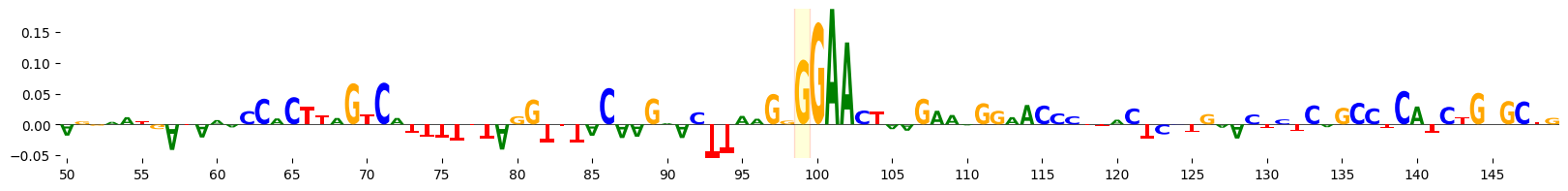
We can visualize the attribution scores for the center of the sequence, highlighting the bases near the variant. Here, we visualize the attributions for the central 100 bp of the 200 bp sequence.

import grelu.visualize
grelu.visualize.plot_attributions(
    ref_attrs, start_pos=50, end_pos=150,
    highlight_positions=[100], ticks=5
)

<logomaker.src.Logo.Logo at 0x7f2b4b8ba4d0>

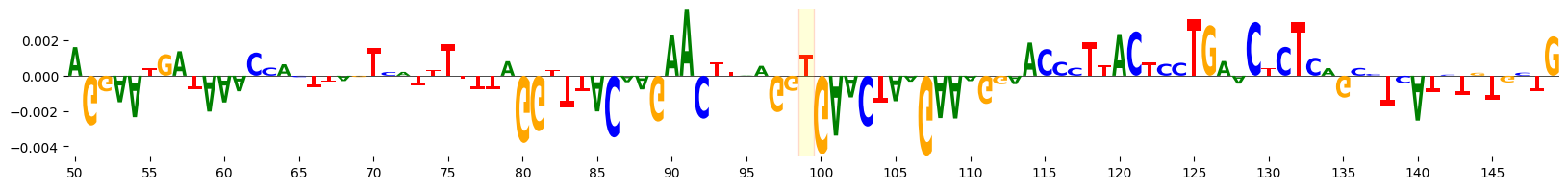
grelu.visualize.plot_attributions(
    alt_attrs, start_pos=50, end_pos=150,
    highlight_positions=[100], ticks=5
)

<logomaker.src.Logo.Logo at 0x7f2b3cee1bd0>

ISM

We can also perform ISM (In silico mutagenesis) of the bases surrounding the variant to see what the effect would be if we mutated the reference allele to any other base. The ISM_predict function in grelu.interpret.score performs every possible single-base substitution on the given sequence, predicts the effect of each substitution, and optionally compares these predictions to the reference sequence to return an effect size for each substitution.

Once again, since we are interested in how important each base is to the model’s prediction in microglia, we use the microglia_score transform. This ensures that ISM will score each base’s importance to the microglial prediction only.

ism = grelu.interpret.score.ISM_predict(
    ref_seq,
    model,
    prediction_transform=microglia_score, # Focus on the prediction in microglia
    compare_func = "log2FC", # Return the log2FC of the mutated sequence prediction w.r.t the reference sequence
    devices=0, # Index of the GPU to use
    num_workers=8,
)

Predicting DataLoader 0: 100%|████████████████████████████████████████████████████████████████████████████████████████████████████████████| 13/13 [00:03<00:00,  3.77it/s]

ism

	C	A	A	A	G	A	T	A	T	A	...	T	T	T	A	G	A	A	A	A	T
A	0.035433	0.000000	0.000000	0.000000	0.176200	0.000000	0.068667	0.000000	0.279563	0.000000	...	0.053832	0.276007	-0.124894	-0.001023	0.096175	-0.001023	-0.001023	-0.001023	-0.001023	0.025681
C	0.000000	0.033218	0.094159	0.089338	0.243149	0.156447	0.097038	0.381914	0.209318	0.283427	...	0.101740	-0.033583	-0.023669	0.073447	-0.123414	0.098240	-0.024329	0.023732	0.075118	0.031927
G	-0.043991	0.028242	0.073336	0.076389	0.000000	0.039801	0.067884	0.356636	0.206355	-0.026990	...	0.012843	-0.067621	-0.116999	-0.055409	-0.001023	0.146642	-0.022481	0.044179	-0.014930	0.024902
T	0.059099	0.051351	0.069703	-0.238775	0.204979	0.038907	0.000000	-0.062656	0.000000	0.224857	...	0.000000	0.000000	-0.001023	-0.034827	0.081750	-0.004022	-0.194302	0.038739	-0.063216	-0.001023

4 rows × 200 columns

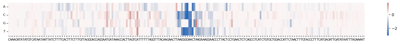
grelu.visualize.plot_ISM(ism, method="heatmap", center=0, figsize=(20, 1.5))

<Axes: >

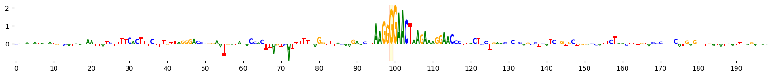
grelu.visualize.plot_ISM(ism, method='logo', figsize=(20, 1.5), highlight_positions=[100])

<logomaker.src.Logo.Logo at 0x7f2b3c821510>

Scan variant with JASPAR consensus motifs

We now scan the sequences immediately around the variant to identify known TF motifs that may have been disrupted by the variant.

# Select the central bases of the sequence
central_ref_seq = grelu.sequence.utils.resize(ref_seq, 18)
central_alt_seq = grelu.sequence.utils.resize(alt_seq, 18)

central_ref_seq, central_alt_seq

('ACTTAAGGGGAACTAAGA', 'ACTTAAGGTGAACTAAGA')

We can use the grelu.interpret.motifs module to scan these sequences with TF motifs. Here, we use a reference set of non-redundant motifs (https://www.vierstra.org/resources/motif_clustering) that are provided with gReLU as consensus.

# Scan with motifs
import grelu.interpret.motifs

scan = grelu.interpret.motifs.compare_motifs(
    ref_seq=central_ref_seq,
    alt_seq=central_alt_seq,
    motifs="consensus",
    pthresh=5e-4,
)

scan

Read 637 motifs from file.

sequence	motif	start	end	strand	alt	ref	foldChange
0	AC0176:MZF:C2H2_ZF	13	6	-	0.000000	9.000000	0.0
1	AC0177:ZNF_MZF:C2H2_ZF	16	5	-	0.000000	8.431193	0.0
2	AC0227:SPI_BCL11A:Ets	5	16	+	0.000000	11.954545	0.0
3	AC0622:ELF_SPIB:Ets	5	14	+	0.000000	8.308943	0.0
4	AC0079:ZNF:C2H2_ZF	14	1	-	1.918367	0.000000	inf

The ref column contains the score for the motif in the reference allele-cintaining sequence and the alt column contains the score in the alternate-allele containing sequence.

Note that the AC0622:ELF_SPIB:Ets motif is lost in the alternate allele-containing sequence.

Compare the variant impact to a background distribution

We saw that the variant has a strong effect size (log2 fold change). To place this effect size in context, we create a set of background sequences by shuffling the sequence surrounding the variant while conserving dinucleotide frequency. We then insert the reference and alternate alleles in each shuffled sequence, and compute the variant effect size again.

test = grelu.variant.marginalize_variants(
    model=model,
    variants=variant.obs,
    genome="hg19",
    prediction_transform=microglia_score,
    seed=0,
    n_shuffles=100,
    compare_func="log2FC",
    rc=True, # Average the result over both strands
)

Predicting variant effects
Predicting DataLoader 0: 100%|██████████████████████████████████████████████████████████████████████████████████████████████████████████████| 1/1 [00:02<00:00,  0.38it/s]
Predicting variant effects in background sequences
Predicting DataLoader 0: 100%|██████████████████████████████████████████████████████████████████████████████████████████████████████████████| 4/4 [00:03<00:00,  1.13it/s]
Calculating background distributions
Performing 2-sided test

test

{'effect_size': [-2.504143476486206],
 'mean': [-0.08852208405733109],
 'sd': [0.4351801872253418],
 'pvalue': [2.8427864717814608e-08]}