Risk profile plot
riskProfile.RdPredictiveness curve, PPV, NPV and 1-NPV risk estimates
Usage
riskProfile(
  outcome,
  score,
  methods = "asis",
  prev.adj = NULL,
  show.prev = TRUE,
  show.nonparam.pv = TRUE,
  show.best.pv = TRUE,
  include = c("PC", "PPV", "1-NPV"),
  plot.raw = FALSE,
  rev.order = FALSE
)
Arguments
- outcome
Vector of binary outcome for each observation.
- score
Numeric vector of continuous predicted risk score.
- methods
-
Character vector of method names (case-insensitive) for plotting curves or a named list where elements are method function and its arguments. Default is set to
"asis".Full options are:
c("asis", "binned", "pava", "mspline", "gam", "cgam").To specify arguments per method, use lists. For example:
list(
  pava = list(method = "pava", ties = "primary"),
  mspline = list(method = "mspline", fitonPerc = TRUE),
  gam = list(method = "gam", bs = "tp", logscores = FALSE),
  bin = list(method = "binned", bins = 10),
  risk = list(method = "asis")
)
See section "Estimation" for more details.
- prev.adj
NULL(default) or scalar numeric between 0 and 1 for prevalence adjustment.- show.prev
Logical, show prevalence value in the graph. Defaults to
TRUE.- show.nonparam.pv
Logical, show non-parametric calculation of PVs. Defaults to
TRUE.- show.best.pv
Logical, show best possible PVs. Defaults to
TRUE.- include
-
Character vector (case-insensitive, partial matching) specifying what quantities to include in the plot.
Default is:
c("PC", "PPV", "1-NPV").Full options are:
c("NPV", "PC", "PPV", "1-NPV"). - plot.raw
Logical to show percentiles or raw values. Defaults to
FALSE(i.e. percentiles).- rev.order
Logical, reverse ordering of scores. Defaults to
FALSE.
Value
A list containing the plot and data, plus errorbar data if they were requested
(through "binned" estimation method with a parameter errorbar.sem).
Estimation
The methods argument specifies the estimation method.
You can provide either a vector of strings, any of
("asis" is not available for calibrationProfile),
or a named list of lists.
In the latter case, the inner list must have an element "method",
which specifies the estimation function (one of those above),
and optionally other elements, which are passed to the estimation function.
For example:
To see what arguments are available for each estimation method,
see the documentation of that function.
The naming convention is getXest,
where X stands for the estimation method, for example getGAMest().
"gam", "cgam", and "mspline" always fit on percentiles by default.
To change this, use fitonPerc = FALSE, for example
"gam" and "cgam" methods are wrappers of mgcv::gam() and cgam::cgam(), respectively.
The default values of function arguments (like k, the number of knots in mgcv::s())
mirror the package defaults.
Examples
# Read in example data
auroc <- read.csv(system.file("extdata", "sample.csv", package = "stats4phc"))
rscore <- auroc$predicted_calibrated
truth <- as.numeric(auroc$actual)
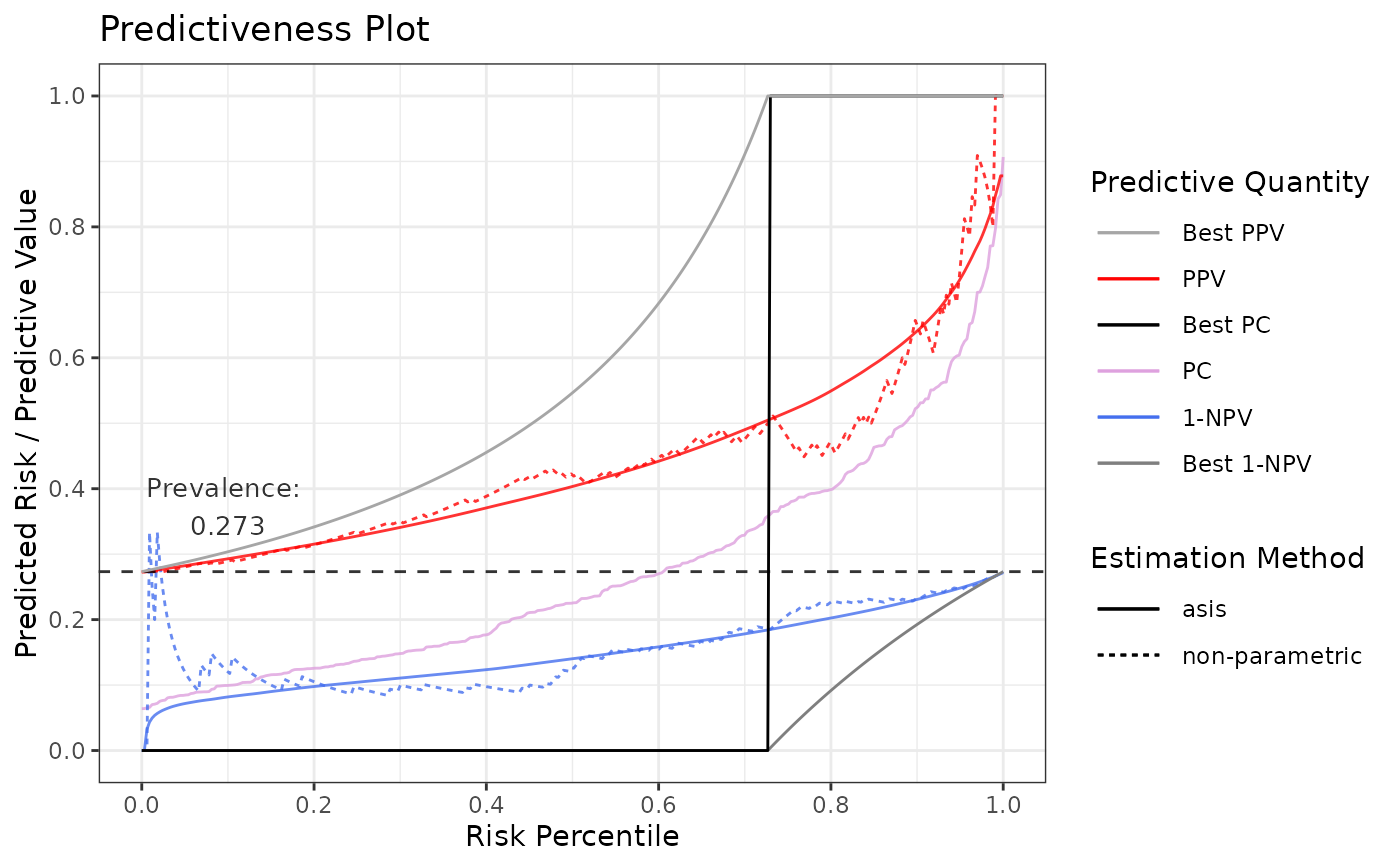
# Default plot includes 1-NPV, PPV, and a predictiveness curve (PC) based on risk-cutoff
p1 <- riskProfile(outcome = truth, score = rscore)
p1$plot
 p1$data
#> # A tibble: 3,340 × 7
#> method score percentile outcome estimate pv pvValue
#> <chr> <dbl> <dbl> <dbl> <dbl> <chr> <dbl>
#> 1 asis NA 0 NA 0.0640 PC NA
#> 2 asis 0.0640 0.00300 0 0.0640 PC NA
#> 3 asis 0.0654 0.00601 0 0.0654 PC NA
#> 4 asis 0.0659 0.00901 1 0.0659 PC NA
#> 5 asis 0.0702 0.0120 0 0.0702 PC NA
#> 6 asis 0.0709 0.0150 0 0.0709 PC NA
#> 7 asis 0.0721 0.0180 1 0.0721 PC NA
#> 8 asis 0.0753 0.0210 0 0.0753 PC NA
#> 9 asis 0.0764 0.0240 0 0.0764 PC NA
#> 10 asis 0.0770 0.0270 0 0.0770 PC NA
#> # ℹ 3,330 more rows
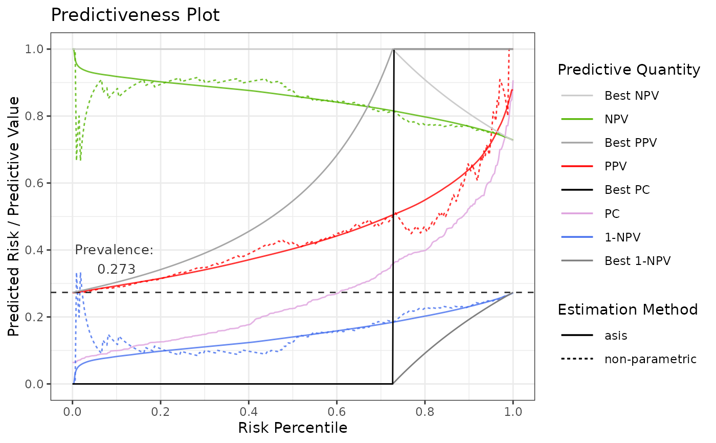
# Show also NPV
p2 <- riskProfile(
outcome = truth,
score = rscore,
include = c("PC", "NPV", "PPV", "1-NPV")
# or use partial matching: include = c("PC", "N", "PPV", "1")
)
p2$plot
p1$data
#> # A tibble: 3,340 × 7
#> method score percentile outcome estimate pv pvValue
#> <chr> <dbl> <dbl> <dbl> <dbl> <chr> <dbl>
#> 1 asis NA 0 NA 0.0640 PC NA
#> 2 asis 0.0640 0.00300 0 0.0640 PC NA
#> 3 asis 0.0654 0.00601 0 0.0654 PC NA
#> 4 asis 0.0659 0.00901 1 0.0659 PC NA
#> 5 asis 0.0702 0.0120 0 0.0702 PC NA
#> 6 asis 0.0709 0.0150 0 0.0709 PC NA
#> 7 asis 0.0721 0.0180 1 0.0721 PC NA
#> 8 asis 0.0753 0.0210 0 0.0753 PC NA
#> 9 asis 0.0764 0.0240 0 0.0764 PC NA
#> 10 asis 0.0770 0.0270 0 0.0770 PC NA
#> # ℹ 3,330 more rows
# Show also NPV
p2 <- riskProfile(
outcome = truth,
score = rscore,
include = c("PC", "NPV", "PPV", "1-NPV")
# or use partial matching: include = c("PC", "N", "PPV", "1")
)
p2$plot
 p2$data
#> # A tibble: 3,674 × 7
#> method score percentile outcome estimate pv pvValue
#> <chr> <dbl> <dbl> <dbl> <dbl> <chr> <dbl>
#> 1 asis NA 0 NA 0.0640 PC NA
#> 2 asis 0.0640 0.00300 0 0.0640 PC NA
#> 3 asis 0.0654 0.00601 0 0.0654 PC NA
#> 4 asis 0.0659 0.00901 1 0.0659 PC NA
#> 5 asis 0.0702 0.0120 0 0.0702 PC NA
#> 6 asis 0.0709 0.0150 0 0.0709 PC NA
#> 7 asis 0.0721 0.0180 1 0.0721 PC NA
#> 8 asis 0.0753 0.0210 0 0.0753 PC NA
#> 9 asis 0.0764 0.0240 0 0.0764 PC NA
#> 10 asis 0.0770 0.0270 0 0.0770 PC NA
#> # ℹ 3,664 more rows
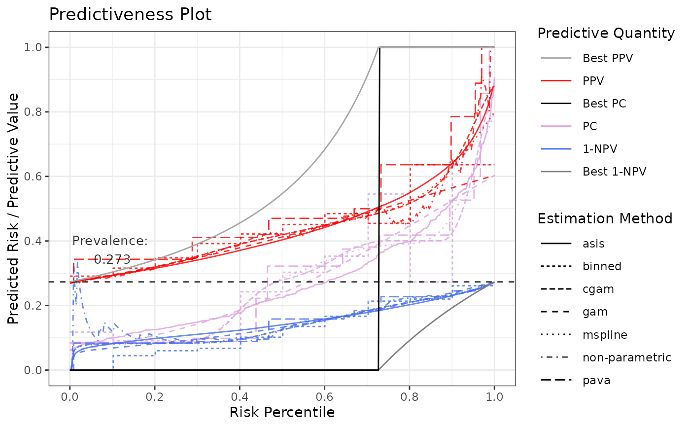
# All estimates of prediction curve
p3 <- riskProfile(
outcome = truth,
score = rscore,
methods = c("mspline", "gam", "cgam", "binned", "pava", "asis"),
include = c("PC", "PPV", "1-NPV")
)
p3$plot
p2$data
#> # A tibble: 3,674 × 7
#> method score percentile outcome estimate pv pvValue
#> <chr> <dbl> <dbl> <dbl> <dbl> <chr> <dbl>
#> 1 asis NA 0 NA 0.0640 PC NA
#> 2 asis 0.0640 0.00300 0 0.0640 PC NA
#> 3 asis 0.0654 0.00601 0 0.0654 PC NA
#> 4 asis 0.0659 0.00901 1 0.0659 PC NA
#> 5 asis 0.0702 0.0120 0 0.0702 PC NA
#> 6 asis 0.0709 0.0150 0 0.0709 PC NA
#> 7 asis 0.0721 0.0180 1 0.0721 PC NA
#> 8 asis 0.0753 0.0210 0 0.0753 PC NA
#> 9 asis 0.0764 0.0240 0 0.0764 PC NA
#> 10 asis 0.0770 0.0270 0 0.0770 PC NA
#> # ℹ 3,664 more rows
# All estimates of prediction curve
p3 <- riskProfile(
outcome = truth,
score = rscore,
methods = c("mspline", "gam", "cgam", "binned", "pava", "asis"),
include = c("PC", "PPV", "1-NPV")
)
p3$plot
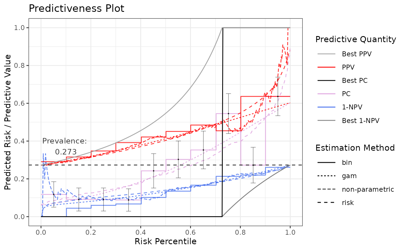
 # Specifying method arguments (note each list has a "method" element)
p4 <- riskProfile(
outcome = truth,
score = rscore,
methods = list(
"gam" = list(method = "gam", bs = "tp", logscores = FALSE, fitonPerc = TRUE),
"risk" = list(method = "asis"), # no available arguments for this method
"bin" = list(method = "binned", quantiles = 10, errorbar.sem = 1.2)
)
)
p4$plot
# Specifying method arguments (note each list has a "method" element)
p4 <- riskProfile(
outcome = truth,
score = rscore,
methods = list(
"gam" = list(method = "gam", bs = "tp", logscores = FALSE, fitonPerc = TRUE),
"risk" = list(method = "asis"), # no available arguments for this method
"bin" = list(method = "binned", quantiles = 10, errorbar.sem = 1.2)
)
)
p4$plot
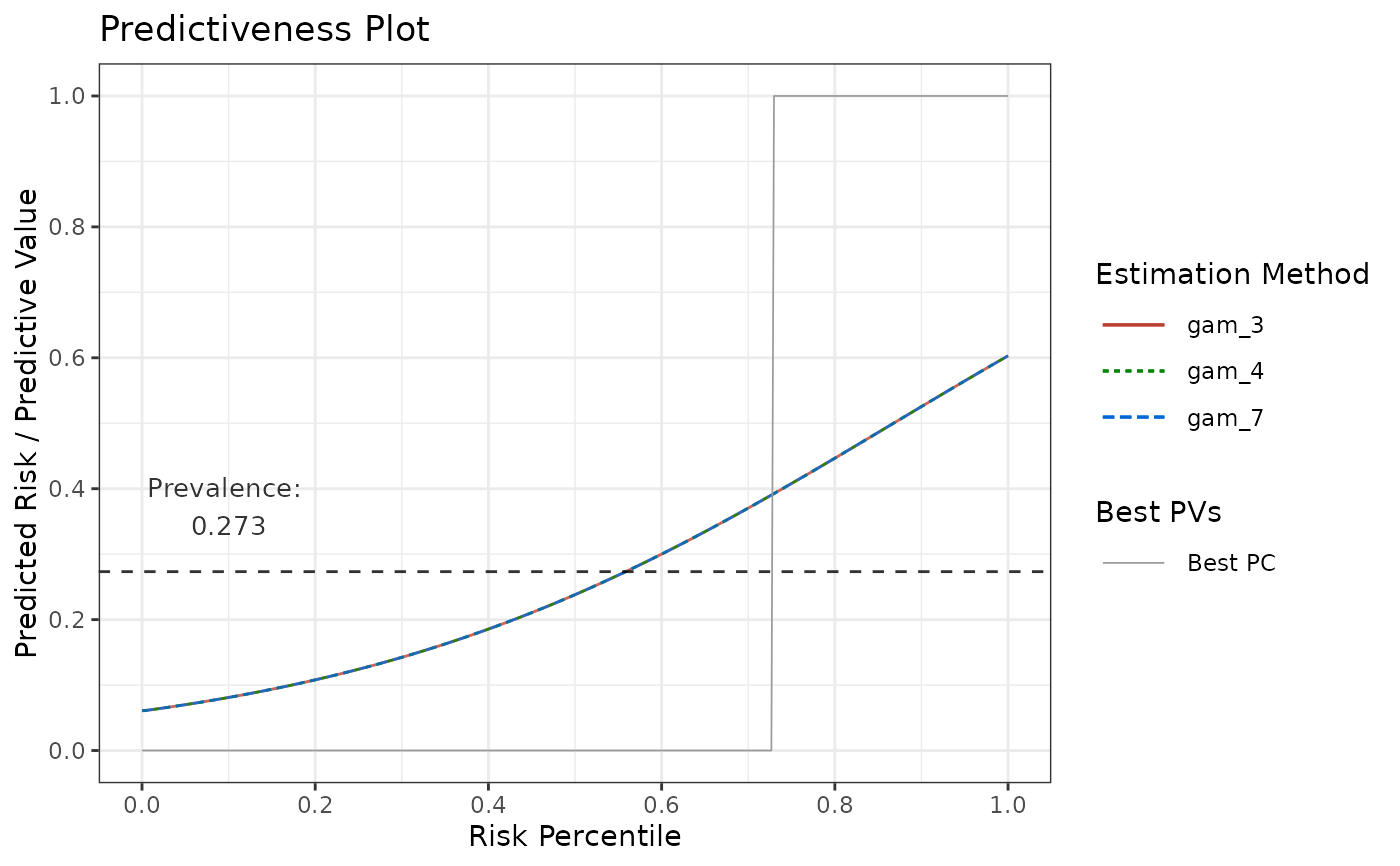
 # Compare multiple GAMs in terms of Predictiveness Curves
p5 <- riskProfile(
outcome = truth,
score = rscore,
methods = list(
"gam_3" = list(method = "gam", k = 3),
"gam_4" = list(method = "gam", k = 4),
"gam_7" = list(method = "gam", k = 7)
),
include = "PC"
)
p5$plot
# Compare multiple GAMs in terms of Predictiveness Curves
p5 <- riskProfile(
outcome = truth,
score = rscore,
methods = list(
"gam_3" = list(method = "gam", k = 3),
"gam_4" = list(method = "gam", k = 4),
"gam_7" = list(method = "gam", k = 7)
),
include = "PC"
)
p5$plot
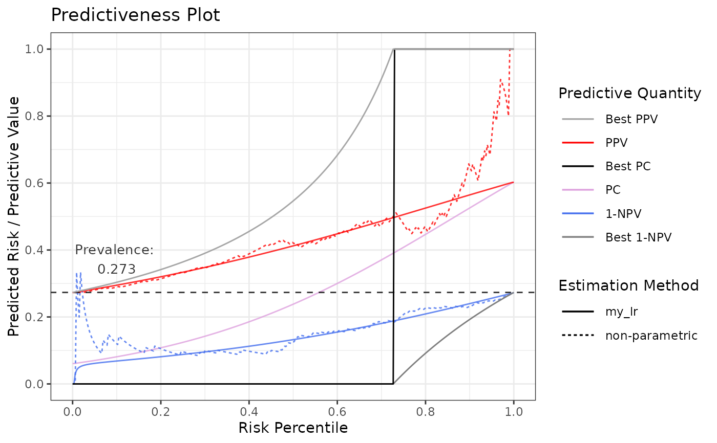
 # Using logistic regression as user-defined estimation function, fitting on percentiles
# Function needs to take exactly these two arguments
my_est <- function(outcome, score) {
# Calculate percentiles
perc <- ecdf(score)(score)
# Fit
m <- glm(outcome ~ perc, family = "binomial")
# Generate predictions
preds <- predict(m, type = "response")
# Return a data.frame with exactly these columns
return(
data.frame(
score = score,
percentile = perc,
outcome = outcome,
estimate = preds
)
)
}
p6 <- riskProfile(
outcome = truth,
score = rscore,
methods = list(my_lr = my_est)
)
p6$plot
# Using logistic regression as user-defined estimation function, fitting on percentiles
# Function needs to take exactly these two arguments
my_est <- function(outcome, score) {
# Calculate percentiles
perc <- ecdf(score)(score)
# Fit
m <- glm(outcome ~ perc, family = "binomial")
# Generate predictions
preds <- predict(m, type = "response")
# Return a data.frame with exactly these columns
return(
data.frame(
score = score,
percentile = perc,
outcome = outcome,
estimate = preds
)
)
}
p6 <- riskProfile(
outcome = truth,
score = rscore,
methods = list(my_lr = my_est)
)
p6$plot
 # Using cgam as user-defined estimation function
# Note that you can also use the predefined cgam using methods = "cgam"
# Attach needed library
# Watch out for masking of mgcv::s and cgam::s if both are attached
library(cgam, quietly = TRUE)
#>
#> Attaching package: ‘cgam’
#> The following objects are masked from ‘package:coneproj’:
#>
#> conc, conv, decr, decr.conc, decr.conv, incr, incr.conc, incr.conv
# Function needs to take exactly these two arguments
my_est <- function(outcome, score) {
# Fit on raw predictions with space = "E"
m <- cgam(
outcome ~ s.incr(score, numknots = 5, space = "E"),
family = "binomial"
)
# Generate predictions and convert to vector
preds <- predict(m, type = "response")$fit
# Return a data.frame with exactly these columns
out <- data.frame(
score = score,
percentile = ecdf(score)(score),
outcome = outcome,
estimate = preds
)
return(out)
}
p7 <- riskProfile(
outcome = truth,
score = rscore,
methods = list(my_cgam = my_est)
)
p7$plot
# Using cgam as user-defined estimation function
# Note that you can also use the predefined cgam using methods = "cgam"
# Attach needed library
# Watch out for masking of mgcv::s and cgam::s if both are attached
library(cgam, quietly = TRUE)
#>
#> Attaching package: ‘cgam’
#> The following objects are masked from ‘package:coneproj’:
#>
#> conc, conv, decr, decr.conc, decr.conv, incr, incr.conc, incr.conv
# Function needs to take exactly these two arguments
my_est <- function(outcome, score) {
# Fit on raw predictions with space = "E"
m <- cgam(
outcome ~ s.incr(score, numknots = 5, space = "E"),
family = "binomial"
)
# Generate predictions and convert to vector
preds <- predict(m, type = "response")$fit
# Return a data.frame with exactly these columns
out <- data.frame(
score = score,
percentile = ecdf(score)(score),
outcome = outcome,
estimate = preds
)
return(out)
}
p7 <- riskProfile(
outcome = truth,
score = rscore,
methods = list(my_cgam = my_est)
)
p7$plot
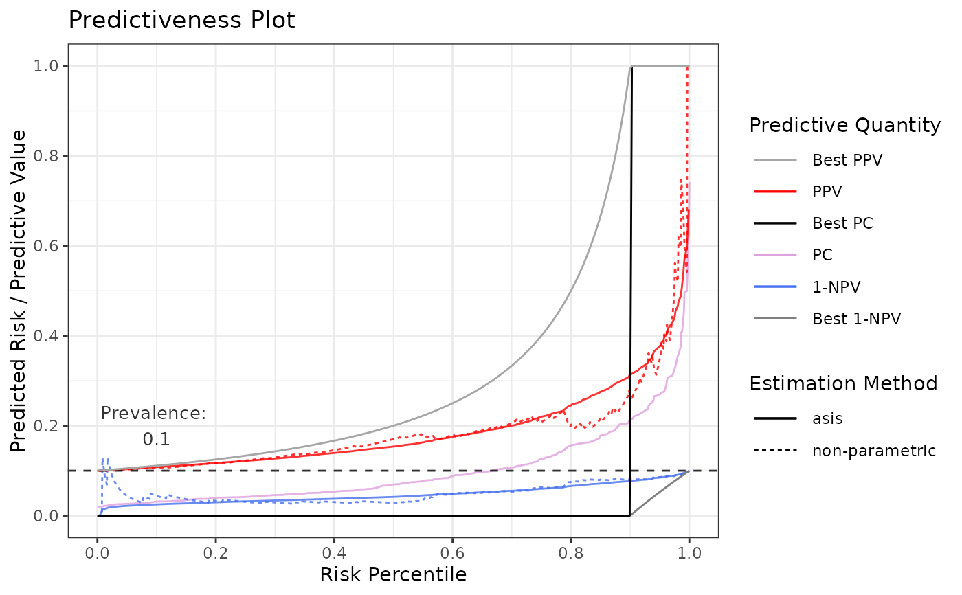
 # Prevalence adjustment to 0.1
p8 <- riskProfile(outcome = truth, score = rscore, prev.adj = 0.1)
p8$plot
# Prevalence adjustment to 0.1
p8 <- riskProfile(outcome = truth, score = rscore, prev.adj = 0.1)
p8$plot