Show the code
library(tidyverse)
library(BayesERtools)
library(posterior)
library(here)
library(gt)

theme_set(theme_bw(base_size = 12))In this section, we will show a basic workflow of performing ER analysis for binary endpoint using the logistic regression model.
library(tidyverse)
library(BayesERtools)
library(posterior)
library(here)
library(gt)
theme_set(theme_bw(base_size = 12))We will use an example simulated dataset included in BayesERtools package (d_sim_binom_cov) for the analysis. In this document we use hypoglycemia (hgly2) as an example AE. Another example AE is diarrhea (dr2), where you would see fairly flat ER curve.
data(d_sim_binom_cov)

head(d_sim_binom_cov) |>
  gt() |>
  fmt_number(n_sigfig = 3) |>
  fmt_integer(columns = c("ID", "AEFLAG", "Dose_mg"))

d_sim_binom_cov_2 <-
  d_sim_binom_cov |>
  mutate(
    AUCss_1000 = AUCss / 1000, BAGE_10 = BAGE / 10,
    BWT_10 = BWT / 10, BHBA1C_5 = BHBA1C / 5,
    Dose = glue::glue("{Dose_mg} mg")
  )

# Grade 2+ hypoglycemia
df_er_ae_hgly2 <- d_sim_binom_cov_2 |> filter(AETYPE == "hgly2")
# Grade 2+ diarrhea
df_er_ae_dr2 <- d_sim_binom_cov_2 |> filter(AETYPE == "dr2")| ID | AETYPE | AEFLAG | Dose_mg | AUCss | Cmaxss | Cminss | BAGE | BWT | BGLUC | BHBA1C | RACE | VISC |
|---|---|---|---|---|---|---|---|---|---|---|---|---|
| 1 | hgly2 | 0 | 200 | 866 | 64.3 | 10.1 | 84.4 | 74.1 | 4.65 | 31.5 | White | No |
| 1 | dr2 | 0 | 200 | 866 | 64.3 | 10.1 | 84.4 | 74.1 | 4.65 | 31.5 | White | No |
| 1 | ae_covsel_test | 0 | 200 | 866 | 64.3 | 10.1 | 84.4 | 74.1 | 4.65 | 31.5 | White | No |
| 2 | hgly2 | 0 | 200 | 1,710 | 166 | 27.3 | 59.1 | 88.2 | 7.24 | 41.9 | White | No |
| 2 | dr2 | 0 | 200 | 1,710 | 166 | 27.3 | 59.1 | 88.2 | 7.24 | 41.9 | White | No |
| 2 | ae_covsel_test | 1 | 200 | 1,710 | 166 | 27.3 | 59.1 | 88.2 | 7.24 | 41.9 | White | No |
We also defines variables that is used in the analysis.
var_resp <- "AEFLAG"
# HbA1c & glucose are only relevant for hyperglycemia
var_cov_ae_hgly2 <-
  c("BAGE_10", "BWT_10", "RACE", "VISC", "BHBA1C_5", "BGLUC")
var_cov_ae_dr2 <-
c("BAGE_10", "BWT_10", "RACE", "VISC")dev_ermod_bin() function can be used to develop basic ER model. (Note that this function can also be used for models with covariates, if you already know the covariates to be included.)
set.seed(1234)
ermod_bin <- dev_ermod_bin(
  data = df_er_ae_hgly2,
  var_resp = var_resp,
  var_exposure = "AUCss_1000"
)
ermod_bin
── Binary ER model ─────────────────────────────────────────────────────────────
ℹ Use `plot_er()` to visualize ER curve

── Developed model ──

stan_glm
 family:       binomial [logit]
 formula:      AEFLAG ~ AUCss_1000
 observations: 500
 predictors:   2
------
            Median MAD_SD
(Intercept) -2.04   0.23
AUCss_1000   0.41   0.08
------
* For help interpreting the printed output see ?print.stanreg
* For info on the priors used see ?prior_summary.stanreg
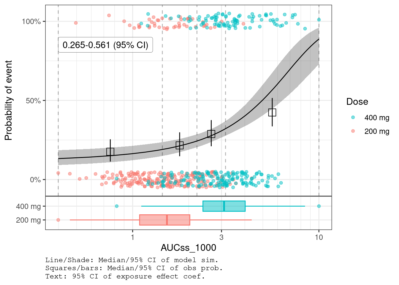
You can compare the observed data with the model fit using plot_er_gof() function.
# Using `*` instead of `+` so that scale can be
# applied for both panels (main plot and boxplot)
plot_er_gof(ermod_bin, var_group = "Dose", show_coef_exp = TRUE) *
  ggplot2::coord_transform(x = "log10") *
  ggplot2::scale_x_continuous(
    breaks = xgxr::xgx_breaks_log10,
    minor_breaks = xgxr::xgx_minor_breaks_log10
  )
MCMC samples can be obtained with as_draws() family of functions, such as as_draws_df().
draws_df <- as_draws_df(ermod_bin)

draws_df_summary <-
  draws_df |>
  summarize_draws(
    mean, median, sd, ~ quantile2(.x, probs = c(0.025, 0.975)),
    default_convergence_measures()
  )

draws_df_summary |>
  gt() |>
fmt_number(n_sigfig = 3)| variable | mean | median | sd | q2.5 | q97.5 | rhat | ess_bulk | ess_tail |
|---|---|---|---|---|---|---|---|---|
| (Intercept) | −2.05 | −2.04 | 0.234 | −2.51 | −1.59 | 1.00 | 2,230 | 1,870 |
| AUCss_1000 | 0.412 | 0.412 | 0.0761 | 0.265 | 0.561 | 1.00 | 2,150 | 2,140 |
You can predict the probability of events for a given exposure level with sim_er_new_exp() function.
Here, the prediction is done for AUCss_1000 of 1, 1.5, 2, 3 (AUCss of 1000, 1500, 2000, 3000), and the output is the median and 95% CI of the predicted probability. You can set output_type = "draw" to get the raw posterior draws.
There are two types of outputs here, .epred and .linpred, as follows:
.epred: Expected response on the probability scale (% of event).linpred: Expected response on the linear predictor scale (logit scale, i.e. log-odds)See ?BayesERtools::sim_er for more details.
ersim_med_qi <- sim_er_new_exp(
  ermod_bin,
  exposure_to_sim_vec = c(1, 1.5, 2, 3),
  output_type = "median_qi"
)
ersim_med_qi |>
  gt() |>
  fmt_number(n_sigfig = 3) |>
fmt_integer(columns = c(".row"))| AUCss_1000 | .row | .epred | .epred.lower | .epred.upper | .linpred | .linpred.lower | .linpred.upper | .width | .point | .interval |
|---|---|---|---|---|---|---|---|---|---|---|
| 1.00 | 1 | 0.164 | 0.122 | 0.213 | −1.63 | −1.97 | −1.31 | 0.950 | median | qi |
| 1.50 | 2 | 0.194 | 0.153 | 0.240 | −1.43 | −1.71 | −1.15 | 0.950 | median | qi |
| 2.00 | 3 | 0.228 | 0.189 | 0.270 | −1.22 | −1.46 | −0.993 | 0.950 | median | qi |
| 3.00 | 4 | 0.308 | 0.266 | 0.354 | −0.811 | −1.02 | −0.603 | 0.950 | median | qi |
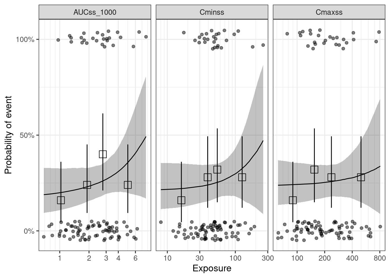
dev_ermod_bin_exp_sel() function can be used to select the best exposure metric(s) from a list of candidate exposure metrics. In this case, AUCss_1000 is selected as the best exposure metric, as it had the highest elpd (expected log predictive density).1
Note that whether you want to select exposure metrics using the statistical criteria (e.g. elpd) or pre-specify the exposure metric(s) depends on the contexts. Should you choose to pre-specify the exposure metric(s), you can skip this step.
set.seed(1234)
ermod_bin_exp_sel <-
  dev_ermod_bin_exp_sel(
    # Use reduced N to make the example run faster
    data = slice_sample(df_er_ae_hgly2, n = 100),
    var_resp = var_resp,
    var_exp_candidates = c("AUCss_1000", "Cmaxss", "Cminss"),
    # Use reduced iter to make the example run faster
    iter = 1000
  )
ℹ The exposure metric selected was: AUCss_1000
ermod_bin_exp_sel
── Binary ER model & exposure metric selection ─────────────────────────────────
ℹ Use `plot_er_exp_sel()` for ER curve of all exposure metrics
ℹ Use `plot_er()` with `show_orig_data = TRUE` for ER curve of the selected exposure metric

── Exposure metrics comparison ──

           elpd_diff se_diff
AUCss_1000  0.00      0.00
Cminss     -0.76      0.70
Cmaxss     -0.91      0.97

── Selected model ──

stan_glm
 family:       binomial [logit]
 formula:      AEFLAG ~ AUCss_1000
 observations: 100
 predictors:   2
------
            Median MAD_SD
(Intercept) -1.59   0.45
AUCss_1000   0.20   0.15
------
* For help interpreting the printed output see ?print.stanreg
* For info on the priors used see ?prior_summary.stanreg
The ER curve for all the evaluated exposure metrics can be generated with plot_er_exp_sel() function.
plot_er_exp_sel(ermod_bin_exp_sel) +
  ggplot2::coord_transform(x = "log10") +
  ggplot2::scale_x_continuous(
    breaks = xgxr::xgx_breaks_log10,
    minor_breaks = xgxr::xgx_minor_breaks_log10
  )
Coordinate system already present.
ℹ Adding new coordinate system, which will replace the existing one.
dev_ermod_bin_cov_sel() function can be used to select the best covariates from a list of candidate covariates. In this case, HbA1c (BHBA1C_5) and glucose (BGLUC) are selected, in addition to the exposure metric AUCss_1000 as predictors.
set.seed(1234)
ermod_bin_cov_sel <-
  dev_ermod_bin_cov_sel(
    data = df_er_ae_hgly2,
    var_resp = var_resp,
    var_exposure = "AUCss_1000",
    var_cov_candidate = var_cov_ae_hgly2,
    verbosity_level = 2
)ermod_bin_cov_sel
── Binary ER model & covariate selection ───────────────────────────────────────
ℹ Use `plot_submod_performance()` to see variable selection performance
ℹ Use `plot_er()` with `marginal = TRUE` to visualize marginal ER curve

── Selected model ──

stan_glm
 family:       binomial [logit]
 formula:      AEFLAG ~ AUCss_1000 + BHBA1C_5 + BGLUC
 observations: 500
 predictors:   4
------
            Median MAD_SD
(Intercept) -11.00   1.12
AUCss_1000    0.49   0.08
BHBA1C_5      0.50   0.09
BGLUC         0.74   0.13
------
* For help interpreting the printed output see ?print.stanreg
* For info on the priors used see ?prior_summary.stanreg
The plot below shows that AUCss_1000, BHBA1C_5, and BGLUC contributes to improving the model performance, and after then the inclusion of no other covariates improves the model performance.
plot_submod_performance(ermod_bin_cov_sel)
In some cases, you might see a warning message like below. This indicates that approximation of leave-one-out cross-validation performance (PSIS-LOO) is not reliable.
Warning: In the recalculation of the reference model's PSIS-LOO CV weights for
the performance evaluation, ... Pareto k-values are in the interval...`.
Alternatively to the default cv_method = "LOO", you can use k-fold cross-validation by settingcv_method = "kfold" in dev_ermod_bin_cov_sel() function. This can take longer time to run, but it can be more reliable in the cases where LOO is not reliable. You can also set validate_search = TRUE to let the function perform the variable selection for each fold separately, rather than using the selected variable sequence from the full dataset evaluation.
set.seed(1234)
ermod_bin_cov_sel_kfold <-
dev_ermod_bin_cov_sel(
data = df_er_ae_hgly2,
var_resp = var_resp,
var_exposure = "AUCss_1000",
var_cov_candidate = var_cov_ae_hgly2,
cv_method = "kfold",
validate_search = TRUE,
verbosity_level = 2
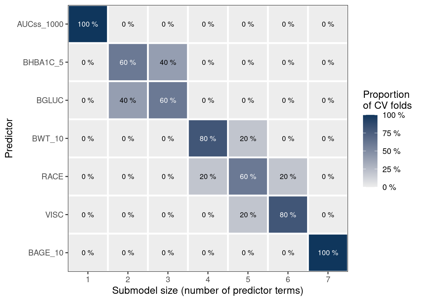
)Added bonus of using k-fold cv is that you can visualize how often each variable is selected in the model. Here, as you can see (and as expected), HbA1c (BHBA1C_5) and glucose (BGLUC) are highly related and they are almost interchangeably selected in the 2nd and 3rd positions. Note that the function enforces the exposure metric to be included first in the model.
ermod_bin_cov_sel_kfold
── Binary ER model & covariate selection ───────────────────────────────────────
ℹ Use `plot_submod_performance()` to see variable selection performance
ℹ Use `plot_var_ranking()` to see variable ranking
ℹ Use `plot_er()` with `marginal = TRUE` to visualize marginal ER curve

── Selected model ──

stan_glm
 family:       binomial [logit]
 formula:      AEFLAG ~ AUCss_1000 + BHBA1C_5 + BGLUC
 observations: 500
 predictors:   4
------
            Median MAD_SD
(Intercept) -10.97   1.20
AUCss_1000    0.49   0.09
BHBA1C_5      0.50   0.09
BGLUC         0.73   0.14
------
* For help interpreting the printed output see ?print.stanreg
* For info on the priors used see ?prior_summary.stanreg
plot_submod_performance(ermod_bin_cov_sel_kfold)
plot_var_ranking(ermod_bin_cov_sel_kfold)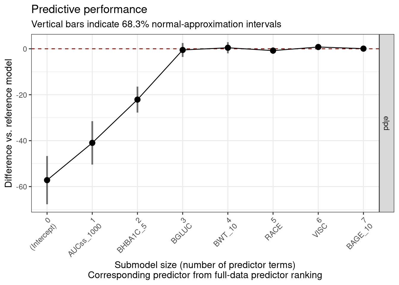
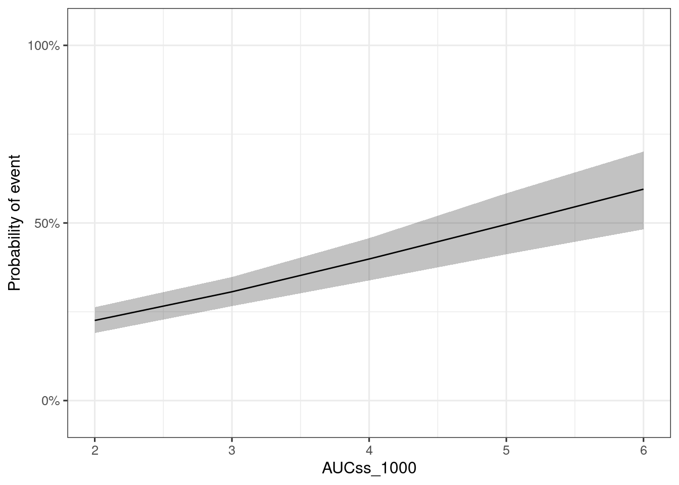
You can simulate the marginal ER relationship, i.e. ER relationships for “marginalized”, or averaged, response for the population of interest, using sim_er_new_exp_marg() function. By default, the covariate distribution is from the original data, but you can also supply other distribution with data_cov argument.
ersim_new_exp_marg_med_qi <- sim_er_new_exp_marg(
  ermod_bin_cov_sel,
  exposure_to_sim_vec = c(2:6),
  output_type = "median_qi"
)
ersim_new_exp_marg_med_qi

plot_er(ersim_new_exp_marg_med_qi, marginal = TRUE)
# A tibble: 5 × 14
.id_exposure AUCss_1000 .epred .epred.lower .epred.upper .linpred
, .linpred.upper ,
# .prediction , .prediction.lower , .prediction.upper ,
# .width , .point , .interval
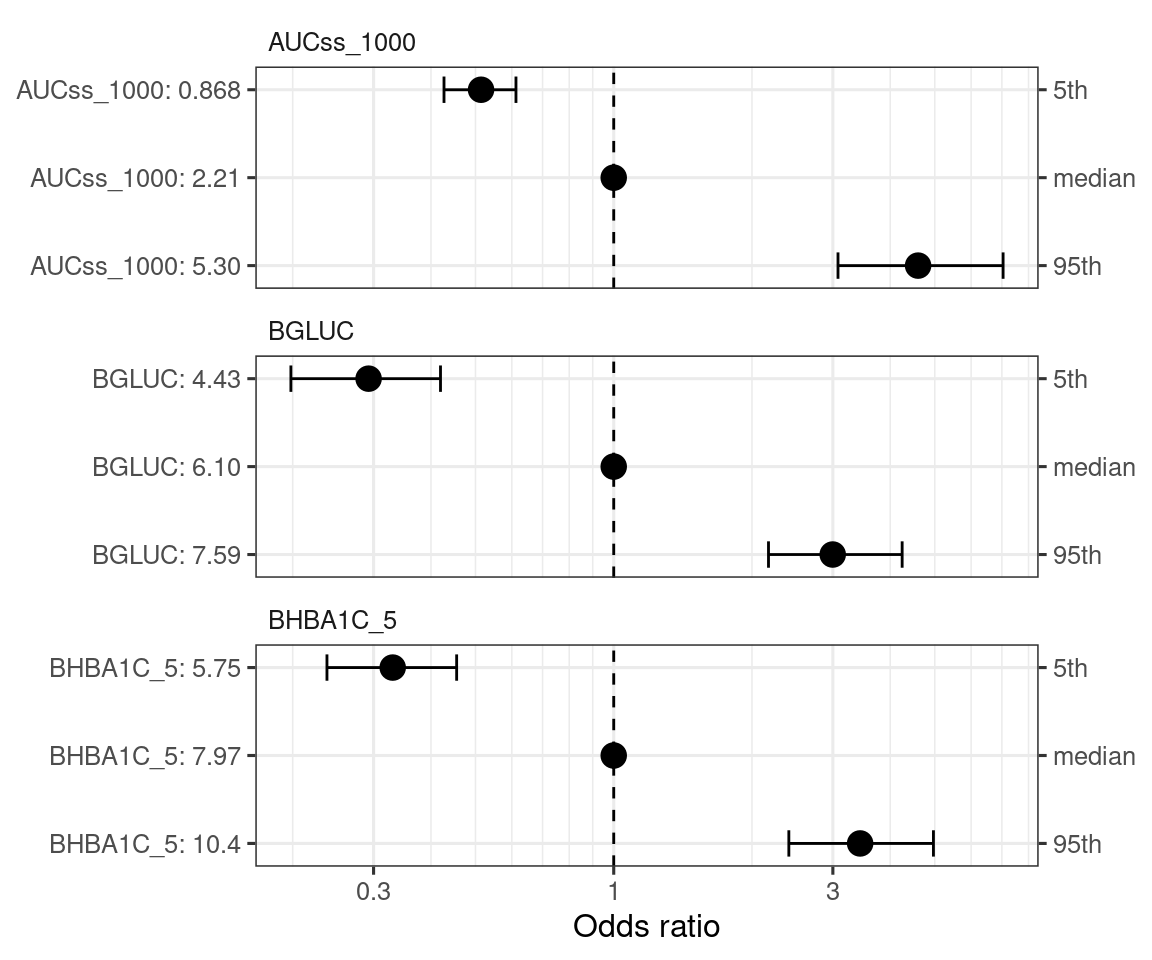
You can visualize the effect of the covariates with sim_coveff() and plot_coveff() functions. You can see that all three predictors have fairly strong effects on the odds ratio of hypoglycemia.
coveffsim <- sim_coveff(ermod_bin_cov_sel)
plot_coveff(coveffsim)
print_coveff(coveffsim)
# A tibble: 9 × 5
var_label value_label value_annot `Odds ratio` `95% CI`
Some references about elpd: , What is the interpretation of ELPD / elpd_loo / elpd_diff?↩︎