6 Workflow without using `BayesERtools`

This page shows how to perform ER analysis without using BayesERtools package to help:

Understand the internal workings of the package
Flexibility to customize the analysis

6.1 Setup and load

Show the code

library(tidyverse)
library(here)
library(gt)

theme_set(theme_bw(base_size = 12))

6.2 Data

Show the code

data(d_sim_binom_cov, package = "BayesERtools")

d_sim_binom_cov_2 <-
  d_sim_binom_cov |>
  mutate(
    AUCss_1000 = AUCss / 1000, BAGE_10 = BAGE / 10,
    BWT_10 = BWT / 10, BHBA1C_5 = BHBA1C / 5
  )

# Grade 2+ hypoglycemia
df_er_ae_hgly2 <- d_sim_binom_cov_2 |> filter(AETYPE == "hgly2")

var_exposure <- "AUCss_1000"
var_resp <- "AEFLAG"
var_cov_ae_hgly2 <- c("BAGE_10", "BWT_10", "RACE", "VISC", "BHBA1C_5", "BGLUC")

6.3 Basic model development

dev_ermod_bin() function can be used to develop basic ER model. (Note that this function can also be used for models with covariates, if you already know the covariates to be included.)

Show the code

set.seed(1234)

var_all <- c(var_exposure) # If you have covariates, you can add here

formula_all <-
  stats::formula(glue::glue(
    "{var_resp} ~ {paste(var_all, collapse = ' + ')}"
  ))

ermod_bin <- rstanarm::stan_glm(
  formula_all,
  family = stats::binomial(),
  data = df_er_ae_hgly2,
  QR = dplyr::if_else(length(var_all) > 1, TRUE, FALSE),
  refresh = 0, # Suppress output
)

ermod_bin

stan_glm
 family:       binomial [logit]
 formula:      AEFLAG ~ AUCss_1000
 observations: 500
 predictors:   2
------
            Median MAD_SD
(Intercept) -2.0    0.2  
AUCss_1000   0.4    0.1  

------
* For help interpreting the printed output see ?print.stanreg
* For info on the priors used see ?prior_summary.stanreg

Perform simulation for plotting purpose

Show the code

exposure_range <-
  range(df_er_ae_hgly2[[var_exposure]])

exposure_to_sim_vec <-
  seq(exposure_range[1], exposure_range[2], length.out = 51)

data_for_sim <- 
  tibble(!!var_exposure := exposure_to_sim_vec)

sim_epred_med_qi <-
  tidybayes::add_epred_draws(data_for_sim, ermod_bin) |>
  tidybayes::median_qi() |>
  dplyr::as_tibble()

Observed vs model predicted plot:

Show the code

ggplot(data = sim_epred_med_qi, aes(x = .data[[var_exposure]], y = .epred)) +
  geom_ribbon(aes(ymin = .lower, ymax = .upper), alpha = 0.3) +
  geom_line() +
  # Observed data plots
  geom_jitter(
    data = df_er_ae_hgly2,
    aes(x = .data[[var_exposure]], y = .data[[var_resp]]),
    width = 0, height = 0.05, alpha = 0.5
  ) +
  xgxr::xgx_stat_ci(
    data = df_er_ae_hgly2,
    aes(x = .data[[var_exposure]], y = .data[[var_resp]]),
    bins = 4, conf_level = 0.95, distribution = "binomial",
    geom = c("point"), shape = 0, size = 4
  ) +
  xgxr::xgx_stat_ci(
    data = df_er_ae_hgly2,
    aes(x = .data[[var_exposure]], y = .data[[var_resp]]),
    bins = 4, conf_level = 0.95, distribution = "binomial",
    geom = c("errorbar"), linewidth = 0.5
  ) +
  # Figure settings
  coord_cartesian(ylim = c(-0.05, 1.05)) +
  scale_y_continuous(
    breaks = c(0, .5, 1),
    labels = scales::percent
  ) +
  labs(x = var_exposure, y = "Probability of event")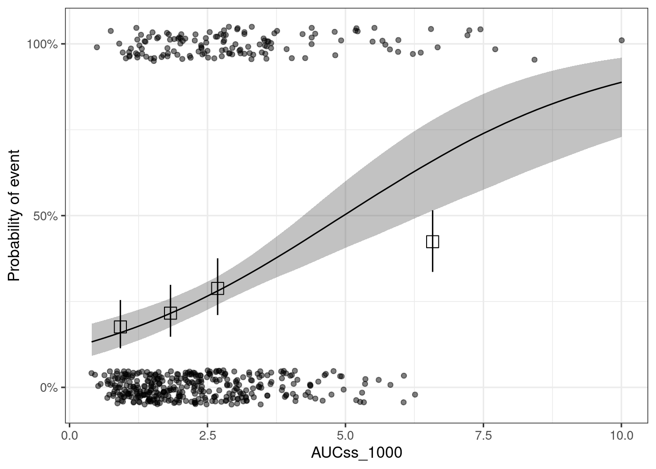

MCMC samples can be obtained with as_draws() family of functions, such as as_draws_df().

Show the code

draws_df <- posterior::as_draws_df(ermod_bin)

draws_df_summary <-
  posterior::summarize_draws(draws_df)

draws_df_summary |>
  gt::gt() |>
  gt::fmt_number(n_sigfig = 3)

variable	mean	median	sd	mad	q5	q95	rhat	ess_bulk	ess_tail
(Intercept)	−2.05	−2.04	0.234	0.228	−2.43	−1.67	1.00	2,230	1,870
AUCss_1000	0.412	0.412	0.0761	0.0765	0.288	0.537	1.00	2,150	2,140

6.4 Selection of exposure metrics

First you fit models with all the candidate exposure metrics and then compare the models using leave-one-out cross-validation (LOO).

Show the code

set.seed(1234)

# Run models with all the candidate exposure metrics
l_mod_exposures <-
  c("AUCss_1000", "Cmaxss", "Cminss") |>
  purrr::set_names() |>
  purrr::map(
    function(.x) {
      formula <- stats::formula(glue::glue("{var_resp} ~ {.x}"))
      
      mod <- rstanarm::stan_glm(
        formula,
        family = stats::binomial(),
        data = df_er_ae_hgly2,
        refresh = 0 # Suppress output
      )
    },
    .progress = TRUE
  )

# Calculate loo (leave-one-out cross-validation) for each model
# and compare the models
l_loo_exposures <- purrr::map(l_mod_exposures, loo::loo)
loo::loo_compare(l_loo_exposures)

           elpd_diff se_diff
AUCss_1000  0.0       0.0   
Cminss     -4.4       3.1   
Cmaxss     -5.1       2.9

6.5 Selection of covariates

Selection of covariates are be done with projpred package in BayesERtools.

6.5.1 Step 1: Full reference model fit

Show the code

varnames <- paste(c(var_exposure, var_cov_ae_hgly2), collapse = " + ")
formula_full <-
  stats::formula(
    glue::glue(
      "{var_resp} ~ {varnames}"
    )
  )

# Need to construct call and then evaluate. Directly calling
# rstanarm::stan_glm with formula_full does not work for the cross-validation
call_fit_ref <-
  rlang::call2(rstanarm::stan_glm,
    formula = formula_full,
    family = quote(stats::binomial()), data = quote(df_er_ae_hgly2), QR = TRUE,
    refresh = 0)
fit_ref <- eval(call_fit_ref)

refm_obj <- projpred::get_refmodel(fit_ref)

6.5.2 Step 2: Variable selection

The code below shows example of variable selection with K-fold cross-validation approach.

Show the code

# Force exposure metric to be always included first
search_terms <- projpred::force_search_terms(
  forced_terms = var_exposure,
  optional_terms = var_cov_ae_hgly2
)

cvvs <- projpred::cv_varsel(
  refm_obj,
  search_terms = search_terms,
  cv_method = "kfold",
  method = "forward",
  validate_search = TRUE,
  refit_prj = TRUE # Evaluation often look strange without refit
)

-----
Running the search using the full dataset ...
10% of terms selected
20% of terms selected
40% of terms selected
50% of terms selected
70% of terms selected
80% of terms selected
100% of terms selected
-----
-----
Refitting the reference model K = 5 times (using the fold-wise training data) ...

Fitting model 1 out of 5

Fitting model 2 out of 5

Fitting model 3 out of 5

Fitting model 4 out of 5

Fitting model 5 out of 5

-----
-----
Running the search and the performance evaluation with `refit_prj = TRUE` for each of the K = 5 CV folds separately ...

  |                                                                            
  |                                                                      |   0%
  |                                                                            
  |==============                                                        |  20%
  |                                                                            
  |============================                                          |  40%
  |                                                                            
  |==========================================                            |  60%
  |                                                                            
  |========================================================              |  80%
  |                                                                            
  |======================================================================| 100%
-----

Show the code

rk <- projpred::ranking(cvvs)

n_var_select <- projpred::suggest_size(cvvs)
n_var_select <- max(1, n_var_select) # At least exposure metric should be included

var_selected <- head(rk[["fulldata"]], n_var_select)

6.5.2.1 Output

Show the code

var_selected

[1] "AUCss_1000" "BHBA1C_5"   "BGLUC"

Show the code

plot(cvvs, text_angle = 45, show_cv_proportions = FALSE, deltas = TRUE)
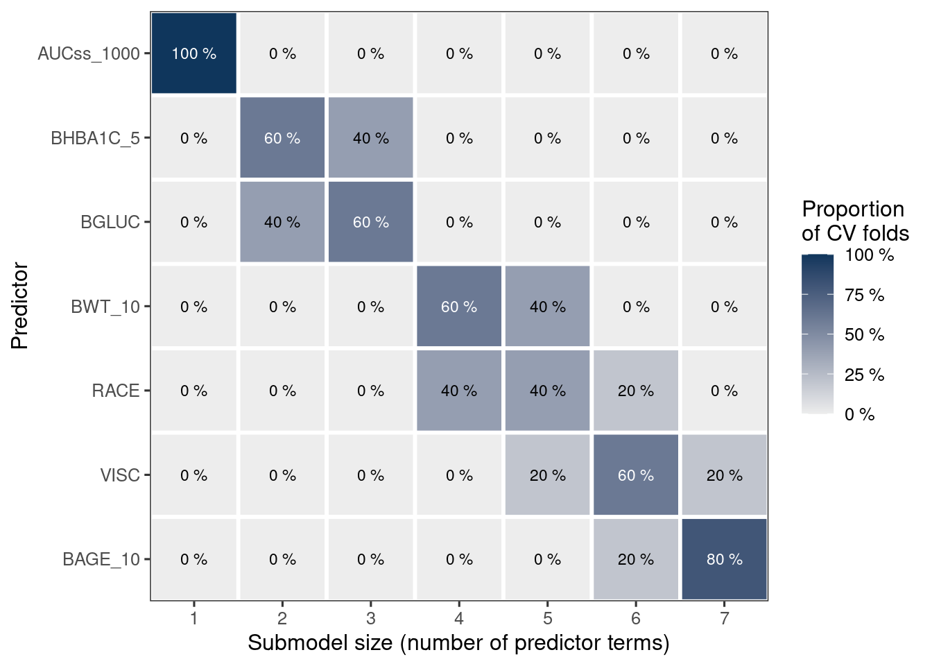
plot(rk) # This only works when cv_method = "kfold" and validate_search = TRUE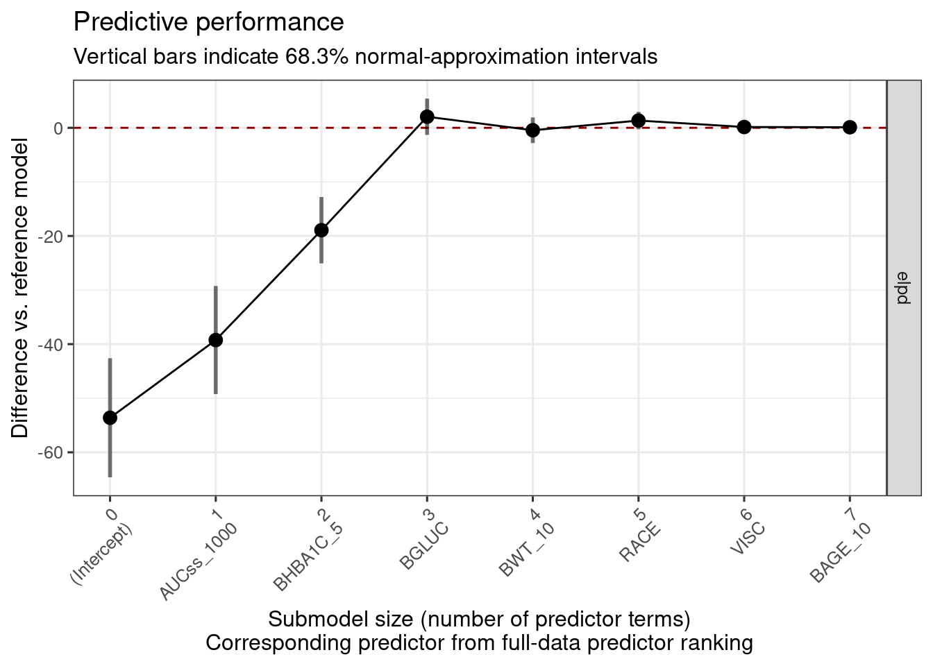

6.5.3 Step 3: Final model fit

Show the code

set.seed(1234)

ermod_bin_cov <- rstanarm::stan_glm(
  stats::formula(glue::glue(
    "{var_resp} ~ {paste(var_selected, collapse = ' + ')}"
  )),
  family = stats::binomial(),
  data = df_er_ae_hgly2,
  QR = dplyr::if_else(length(var_selected) > 1, TRUE, FALSE),
  refresh = 0, # Suppress output
)

ermod_bin_cov

stan_glm
 family:       binomial [logit]
 formula:      AEFLAG ~ AUCss_1000 + BHBA1C_5 + BGLUC
 observations: 500
 predictors:   4
------
            Median MAD_SD
(Intercept) -11.0    1.2 
AUCss_1000    0.5    0.1 
BHBA1C_5      0.5    0.1 
BGLUC         0.7    0.1 

------
* For help interpreting the printed output see ?print.stanreg
* For info on the priors used see ?prior_summary.stanreg

6.6 Marginal ER prediction

The example below simulate the marginal ER relationship, i.e. ER relationships for “marginalized”, or averaged, response for the population of interest, using the covariate distribution is from the original data.

Show the code

exposure_to_sim <- c(2:6)

data_cov <- df_er_ae_hgly2 |> select(-!!var_exposure)

data_for_sim <- 
  tibble(!!var_exposure := exposure_to_sim) |>
  mutate(.id_exposure = row_number()) |>
  expand_grid(data_cov)

sim_epred_raw <-
  tidybayes::add_epred_draws(data_for_sim, ermod_bin_cov)

# Calculate marginal expected response for each exposure value and draw
sim_epred_marg <-
  sim_epred_raw |>
  dplyr::ungroup() |>
  dplyr::summarize(
    .epred = mean(.epred),
    .by = c(.id_exposure, !!var_exposure, .draw)
  )

sim_epred_marg_med_qi <-
  sim_epred_marg |>
  dplyr::group_by(.id_exposure, !!sym(var_exposure)) |>
  tidybayes::median_qi() |>
  dplyr::as_tibble()

sim_epred_marg_med_qi |>
  gt::gt() |>
  gt::fmt_number(n_sigfig = 3) |>
  gt::fmt_integer(columns = c(".id_exposure"))

.id_exposure	AUCss_1000	.epred	.lower	.upper	.width	.point	.interval
1	2.00	0.228	0.192	0.267	0.950	median	qi
2	3.00	0.307	0.268	0.347	0.950	median	qi
3	4.00	0.396	0.341	0.455	0.950	median	qi
4	5.00	0.491	0.409	0.576	0.950	median	qi
5	6.00	0.588	0.477	0.692	0.950	median	qi