5  Customize covariate effect plots

This page showcase how to customize the covariate effect plots.

5.1 Setup and load

library(tidyverse)
library(BayesERtools)
library(here)
library(gt)

theme_set(theme_bw(base_size = 12))

5.2 Load data

data(d_sim_binom_cov)

d_sim_binom_cov_2 <-
  d_sim_binom_cov |>
  mutate(
    AUCss_1000 = AUCss / 1000, BAGE_10 = BAGE / 10,
    BWT_10 = BWT / 10, BHBA1C_5 = BHBA1C / 5
  )

# Grade 2+ hypoglycemia
df_er_ae_hgly2 <- d_sim_binom_cov_2 |> filter(AETYPE == "hgly2")

var_resp <- "AEFLAG"
var_exposure <- "AUCss_1000"

5.3 Fit model

set.seed(1234)
ermod_bin_hgly2_cov <- dev_ermod_bin(
  data = df_er_ae_hgly2,
  var_resp = var_resp,
  var_cov = c("RACE", "BGLUC", "BHBA1C_5"),
  var_exposure = var_exposure
)

5.4 Evaluation of covariate effects

By default, the covariate effect plots are generated for 5th and 95th percentiles of the continuous covariates and for each level of the categorical covariates (in the order of frequency in data).

coveffsim <- sim_coveff(ermod_bin_hgly2_cov)
plot_coveff(coveffsim)

Figure 5.1

You can modify the width of the quantile interval using the qi_width_cov argument.

coveffsim_qicov_08 <- sim_coveff(ermod_bin_hgly2_cov, qi_width_cov = 0.8)
plot_coveff(coveffsim_qicov_08)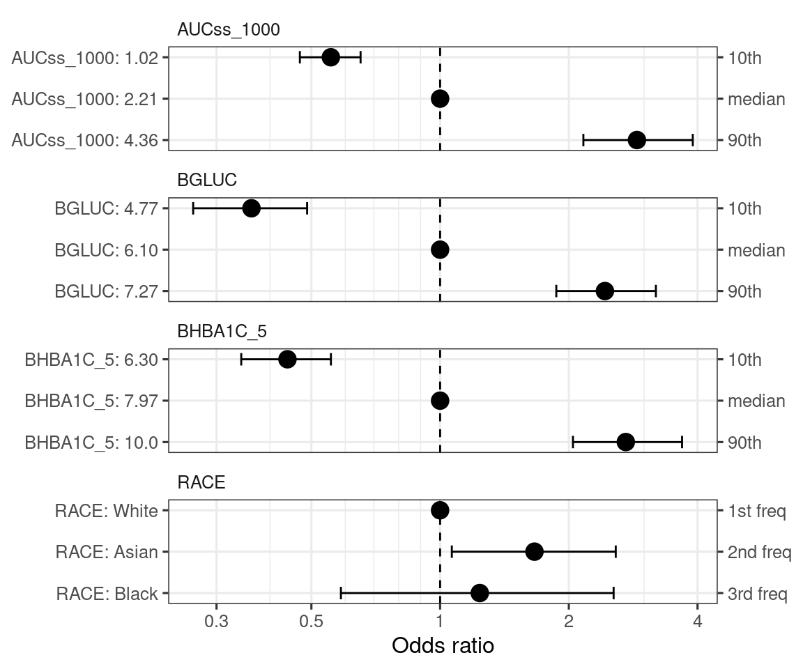

Figure 5.2

5.5 Further customization

These covariate effect simulation (and plotting) can be customized by providing specifications to sim_coveff() function.

First, we build the specification for the covariate effects with build_spec_coveff() function.

spec_coveff <- build_spec_coveff(ermod_bin_hgly2_cov)
spec_coveff |> 
  gt() |> 
  fmt_number(n_sigfig = 3)|>
  fmt_integer(columns = c("value_order", "var_order"))

var_order	var_name	var_label	value_order	value_annot	value_label	value_cont	value_cat	is_ref_value	show_ref_value	is_covariate
1	AUCss_1000	AUCss_1000	1	5th	0.868	0.868	NA	FALSE	NA	FALSE
1	AUCss_1000	AUCss_1000	2	median	2.21	2.21	NA	TRUE	TRUE	FALSE
1	AUCss_1000	AUCss_1000	3	95th	5.30	5.30	NA	FALSE	NA	FALSE
2	RACE	RACE	1	1st freq	White	NA	White	TRUE	TRUE	TRUE
2	RACE	RACE	2	2nd freq	Asian	NA	Asian	FALSE	NA	TRUE
2	RACE	RACE	3	3rd freq	Black	NA	Black	FALSE	NA	TRUE
3	BGLUC	BGLUC	1	5th	4.43	4.43	NA	FALSE	NA	TRUE
3	BGLUC	BGLUC	2	median	6.10	6.10	NA	TRUE	TRUE	TRUE
3	BGLUC	BGLUC	3	95th	7.59	7.59	NA	FALSE	NA	TRUE
4	BHBA1C_5	BHBA1C_5	1	5th	5.75	5.75	NA	FALSE	NA	TRUE
4	BHBA1C_5	BHBA1C_5	2	median	7.97	7.97	NA	TRUE	TRUE	TRUE
4	BHBA1C_5	BHBA1C_5	3	95th	10.4	10.4	NA	FALSE	NA	TRUE

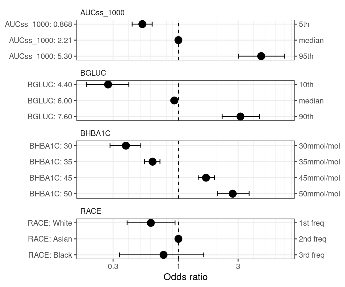
Let’s say we want to customize in a follwoing way:

• Re-calculate percentiles of BGLUC from new distribution (example below uses uniform distribution between 4 and 8) and change the width of the quantile interval to 0.8.
• Use specific values for BHBA1C (30, 35, 45, 50) and label with the original scale rather than those devided by 5 (used in the model).
• Use Asian as the reference level
• Show the plots in the order of BGLUC, BHBA1C, and then RACE

spec_new_bgluc <- build_spec_coveff_one_variable(
  "BGLUC", seq(4, 8, by = 0.1),
  qi_width_cov = 0.8, show_ref_value = TRUE
)

spec_new_bhba1c <- 
  tibble(value_cont = c(30, 35, 45, 50) / 5) |> 
  mutate(
    value_order = row_number(),
    value_label = as.character(value_cont * 5),
    var_name = "BHBA1C_5",
    var_label = "BHBA1C",
    value_annot = glue::glue("{value_label}mmol/mol"),
    is_ref_value = FALSE,
    show_ref_value = FALSE)

spec_new_race <- 
  spec_coveff |> 
  filter(var_name == "RACE") |> 
  mutate(
    is_ref_value = c(FALSE, TRUE, FALSE),
    show_ref_value = c(FALSE, TRUE, FALSE)
  ) |> 
  select(-var_order, -is_covariate)

spec_coveff_new_1 <- 
  replace_spec_coveff(spec_coveff, bind_rows(spec_new_bgluc, spec_new_bhba1c)) |>
  # spec_new_race is separately provided as we want to change the reference level
  replace_spec_coveff(spec_new_race, replace_ref_value = TRUE)

d_new_var_order <- 
  tibble(var_name = c("AUCss_1000", "BGLUC", "BHBA1C_5", "RACE")) |> 
  mutate(var_order = row_number())

spec_coveff_new <- 
  spec_coveff_new_1 |> 
  select(-var_order) |>
  left_join(d_new_var_order, by = "var_name")

spec_coveff_new |> 
  gt() |> 
  fmt_number(n_sigfig = 3)|>
  fmt_integer(columns = c("value_order", "var_order"))

var_name	value_order	value_annot	value_label	value_cont	value_cat	is_ref_value	show_ref_value	var_label	is_covariate	var_order
AUCss_1000	1	5th	0.868	0.868	NA	FALSE	NA	AUCss_1000	FALSE	1
AUCss_1000	2	median	2.21	2.21	NA	TRUE	TRUE	AUCss_1000	FALSE	1
AUCss_1000	3	95th	5.30	5.30	NA	FALSE	NA	AUCss_1000	FALSE	1
RACE	1	1st freq	White	NA	White	FALSE	FALSE	RACE	TRUE	4
RACE	2	2nd freq	Asian	NA	Asian	TRUE	TRUE	RACE	TRUE	4
RACE	3	3rd freq	Black	NA	Black	FALSE	FALSE	RACE	TRUE	4
BGLUC	1	NA	6.10	6.10	NA	TRUE	FALSE	BGLUC	TRUE	2
BGLUC	2	10th	4.40	4.40	NA	FALSE	NA	BGLUC	TRUE	2
BGLUC	3	median	6.00	6.00	NA	FALSE	NA	BGLUC	TRUE	2
BGLUC	4	90th	7.60	7.60	NA	FALSE	NA	BGLUC	TRUE	2
BHBA1C_5	1	NA	7.97	7.97	NA	TRUE	FALSE	BHBA1C	TRUE	3
BHBA1C_5	2	30mmol/mol	30	6.00	NA	FALSE	NA	BHBA1C	TRUE	3
BHBA1C_5	3	35mmol/mol	35	7.00	NA	FALSE	NA	BHBA1C	TRUE	3
BHBA1C_5	4	45mmol/mol	45	9.00	NA	FALSE	NA	BHBA1C	TRUE	3
BHBA1C_5	5	50mmol/mol	50	10.0	NA	FALSE	NA	BHBA1C	TRUE	3

The customized covariate effect plots can be generated using the plot_coveff()

coveffsim_spec <- sim_coveff(ermod_bin_hgly2_cov, spec_coveff = spec_coveff_new)
plot_coveff(coveffsim_spec)

Figure 5.3