In this section, we will show a basic workflow for performing an Emax model analysis for continuous endpoint.

7.1 Setup and load

Show the code
library(tidyverse)
library(BayesERtools)
library(posterior)
library(tidybayes)
library(here)
library(gt)

theme_set(theme_bw(base_size = 12))

7.2 Load data

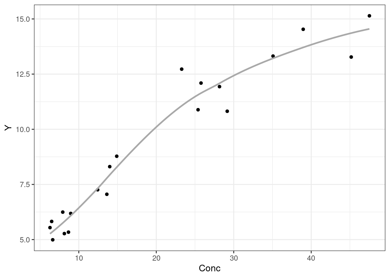
The data for the example is included in the BayesERtools package, which contains a simulated data set d_sim_emax. The analysis uses the exposure variable to predict the continuous outcome response_1. The data are illustrated below:

Show the code
d_sim_emax |>
  head() |>
  gt() |>
  fmt_number(decimals = 2)

```{=html}
dose exposure response_1 response_2 cnt_a cnt_b cnt_c bin_d bin_e
100.00 4,151.15 12.80 1.00 5.71 2.33 7.83 0.00 1.00
100.00 8,067.26 14.58 1.00 4.92 4.66 6.74 1.00 1.00
100.00 4,877.67 12.76 1.00 4.88 4.21 4.68 1.00 1.00
100.00 9,712.93 16.55 1.00 8.42 6.56 1.29 0.00 1.00
100.00 11,490.74 14.41 0.00 4.37 3.96 3.55 0.00 1.00
100.00 2,451.55 12.60 1.00 8.69 7.60 3.64 0.00 0.00
```
Figure 7.1
Show the code
ggplot(d_sim_emax, aes(exposure, response_1)) +
  geom_point() +
  geom_smooth(
    formula = y ~ x, 
    method = "loess", 
    se = FALSE, 
    col = "darkgrey"
  )
Figure 7.2

7.3 Sigmoidal Emax model

Show the code
set.seed(1234)

ermod_sigemax <- dev_ermod_emax(
  data = d_sim_emax,
  var_resp = "response_1",
  var_exposure = "exposure",
  gamma_fix = NULL
)

ermod_sigemax

── Emax model ──────────────────────────────────────────────────────────────────
 Use `plot_er()` to visualize ER curve

── Developed model ──

---- Emax model fit with rstanemax ----
         mean se_mean      sd   2.5%     25%     50%     75%    97.5%   n_eff
emax    11.59    0.31    5.89   4.82    7.34   10.10   14.24    27.50  368.24
e0       6.68    0.20    4.08  -3.67    4.78    7.68    9.71    11.48  436.14
ec50  5254.72  193.00 4475.71 801.17 2974.18 4673.97 6385.68 15736.00  537.81
gamma    1.06    0.02    0.50   0.32    0.70    0.97    1.33     2.26  543.20
sigma    1.27    0.00    0.05   1.18    1.24    1.27    1.31     1.39 1375.87
      Rhat
emax  1.01
e0    1.01
ec50  1.00
gamma 1.01
sigma 1.00
* Use `extract_stanfit()` function to extract raw stanfit object
* Use `extract_param()` function to extract posterior draws of key parameters
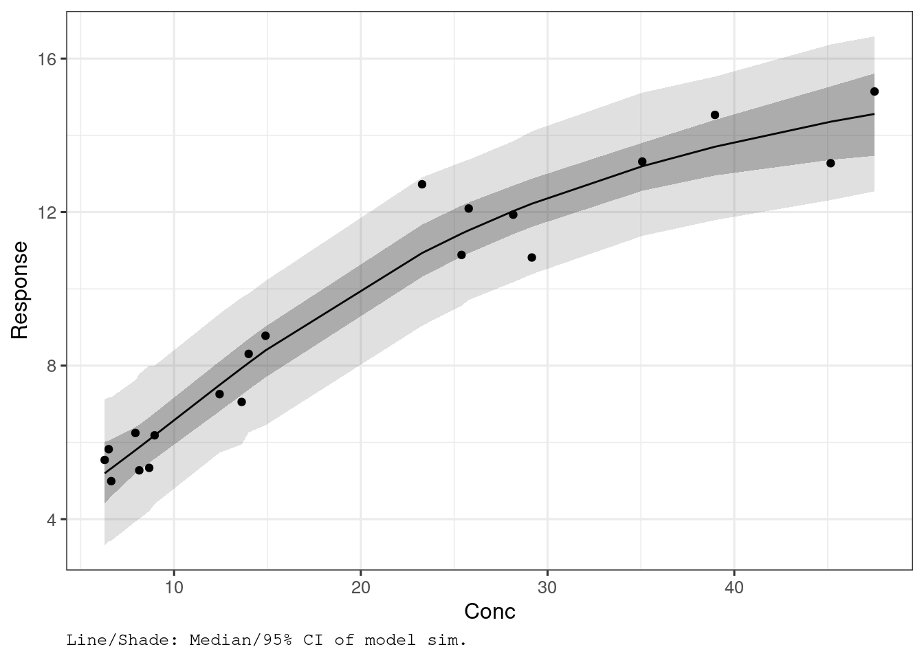
* Use `plot()` function to visualize model fit
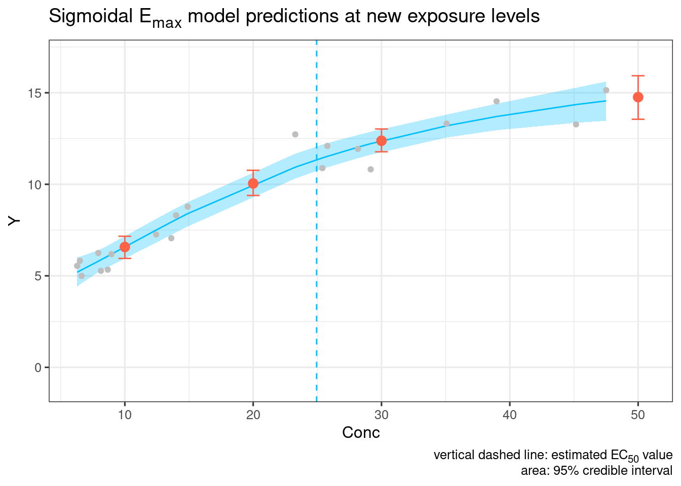
* Use `posterior_predict()` or `posterior_predict_quantile()` function to get
  raw predictions or make predictions on new data
* Use `extract_obs_mod_frame()` function to extract raw data 
  in a processed format (useful for plotting)

7.4 Observation vs model fit

Show the code
d_sim_ermod_sigemax <-
  sim_er(ermod_sigemax, output_type = c("median_qi"))

plot_er_gof(d_sim_ermod_sigemax)
Figure 7.3

7.5 Parameter estimates

Show the code
d_draws_sigemax <- as_draws_df(ermod_sigemax)

d_draws_sigemax_summary <-
  summarize_draws(d_draws_sigemax)

ec50_mean <-
  d_draws_sigemax_summary |>
  filter(variable == "ec50") |>
  pull(mean)

d_draws_sigemax_summary |>
  gt() |>
  fmt_number(decimals = 2)

```{=html}
variable mean median sd mad q5 q95 rhat ess_bulk ess_tail
ec50 5,254.72 4,673.97 4,475.71 2,534.11 1,125.57 9,837.30 1.01 614.40 541.30
sigma 1.27 1.27 0.05 0.05 1.19 1.36 1.00 1,379.24 1,505.63
gamma 1.06 0.97 0.50 0.45 0.40 2.04 1.01 459.99 555.58
e0 6.68 7.68 4.08 3.42 −1.45 11.20 1.01 480.68 788.66
emax 11.59 10.10 5.89 4.79 5.20 23.06 1.01 429.41 533.51
```

7.6 Prediction at a certain concentrations

Show the code
d_sim_new_conc <-
  sim_er_new_exp(ermod_sigemax,
    exposure_to_sim_vec  = c(5000, 15000, 25000, 35000),
    output_type = c("median_qi"))

d_sim_new_conc |>
  select(-starts_with(".linpred"), -c(.row, .width, .point, .interval)) |>
  gt() |>
  fmt_number(decimals = 2) |>
  tab_header(
    title = md("Prediction at specific concentrations")
  )

```{=html}
Prediction at specific concentrations
exposure .epred .epred.lower .epred.upper .prediction .prediction.lower .prediction.upper
5,000.00 13.05 12.79 13.30 13.04 10.49 15.57
15,000.00 15.33 15.12 15.54 15.36 12.86 17.85
25,000.00 16.05 15.75 16.36 16.05 13.57 18.56
35,000.00 16.40 15.91 16.95 16.42 13.83 18.92
```
Figure 7.4
Show the code
d_sim_ermod_sigemax |>
  ggplot(aes(x = exposure, y = response_1)) +
  # Emax model curve
  geom_vline(
    xintercept = ec50_mean, 
    linetype = "dashed", 
    color = "deepskyblue"
  ) +
  geom_ribbon(
    mapping = aes(
      y = .epred, 
      ymin = .epred.lower, 
      ymax = .epred.upper
    ),
    alpha = 0.3, 
    fill = "deepskyblue"
  ) +
  geom_line(
    mapping = aes(y = .epred), 
    color = "deepskyblue"
  ) +
  # Observed data
  geom_point(
    data = d_sim_emax, 
    color = "grey"
  ) +
  # Prediction at the specified doses
  geom_point(
    data = d_sim_new_conc, 
    mapping = aes(y = .epred), 
    color = "tomato", 
    size = 3
  ) +
  geom_errorbar(
    data = d_sim_new_conc,
    mapping = aes(
      y = .epred, 
      ymin = .epred.lower, 
      ymax = .epred.upper
    ),
    width = 1, 
    color = "tomato"
  ) +
  coord_cartesian(ylim = c(7, 21)) +
  scale_fill_brewer(palette = "Greys") +
  labs(
    title = "Sigmoidal E~max~ model predictions at new exposure levels",
    caption = paste(
      "vertical dashed line: estimated EC~50~ value",
      "area: 95% credible interval", 
      sep = "<br>"
    )
  ) +
  theme(
    plot.title = ggtext::element_markdown(),
    plot.caption = ggtext::element_markdown()
  )
Figure 7.5