4  Model comparison between linear and E_max

This page showcase how to compare model structures between linear and E_max logistic regression models

4.1 Setup and load

library(tidyverse)
library(BayesERtools)
library(loo)
library(here)
library(gt)

theme_set(theme_bw(base_size = 12))

4.2 Load data

data(d_sim_binom_cov)

d_sim_binom_cov_2 <-
  d_sim_binom_cov |>
  mutate(
    AUCss_1000 = AUCss / 1000, BAGE_10 = BAGE / 10,
    BWT_10 = BWT / 10, BHBA1C_5 = BHBA1C / 5,
    Dose = glue::glue("{Dose_mg} mg")
  )

# Grade 2+ hypoglycemia
df_er_ae_hgly2 <- d_sim_binom_cov_2 |> filter(AETYPE == "hgly2")

var_resp <- "AEFLAG"
var_exposure <- "AUCss_1000"

4.3 Fit model

Linear logistic regression

set.seed(1234)
ermod_bin_hgly2 <- dev_ermod_bin(
  data = df_er_ae_hgly2,
  var_resp = var_resp,
  var_exposure = var_exposure
)
ermod_bin_hgly2

── Binary ER model ─────────────────────────────────────────────────────────────
ℹ Use `plot_er()` to visualize ER curve

── Developed model ──

stan_glm
 family:       binomial [logit]
 formula:      AEFLAG ~ AUCss_1000
 observations: 500
 predictors:   2
------
            Median MAD_SD
(Intercept) -2.04   0.23 
AUCss_1000   0.41   0.08 
------
* For help interpreting the printed output see ?print.stanreg
* For info on the priors used see ?prior_summary.stanreg

plot_er_gof(ermod_bin_hgly2, var_group = "Dose")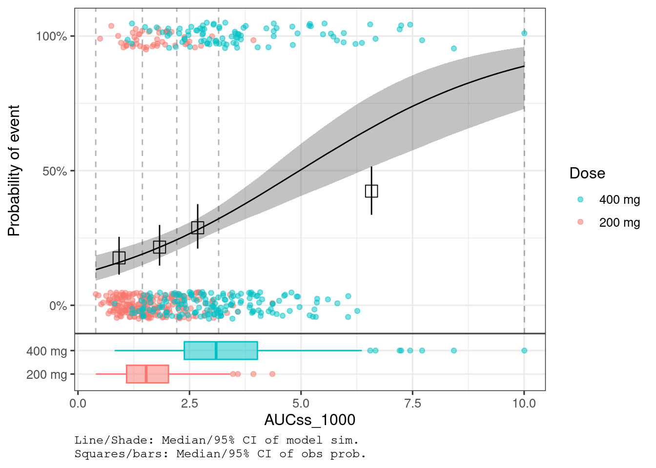

Figure 4.1

Emax logistic regression

set.seed(1234)
ermod_bin_emax_hgly2 <- dev_ermod_bin_emax(
  data = df_er_ae_hgly2,
  var_resp = var_resp,
  var_exposure = var_exposure
)
ermod_bin_emax_hgly2

── Binary Emax model ───────────────────────────────────────────────────────────
ℹ Use `plot_er()` to visualize ER curve

── Developed model ──

---- Binary Emax model fit with rstanemax ----
       mean se_mean   sd  2.5%   25%   50%   75% 97.5%   n_eff Rhat
emax   4.09    0.02 0.94  2.29  3.45  4.04  4.68  6.05 1488.73    1
e0    -2.36    0.01 0.43 -3.33 -2.61 -2.32 -2.07 -1.66 1371.53    1
ec50   4.93    0.06 2.18  1.51  3.32  4.68  6.27  9.79 1431.19    1
gamma  1.00     NaN 0.00  1.00  1.00  1.00  1.00  1.00     NaN  NaN
* Use `extract_stanfit()` function to extract raw stanfit object
* Use `extract_param()` function to extract posterior draws of key parameters
* Use `plot()` function to visualize model fit
* Use `extract_obs_mod_frame()` function to extract raw data 
  in a processed format (useful for plotting)

plot_er_gof(ermod_bin_emax_hgly2, var_group = "Dose")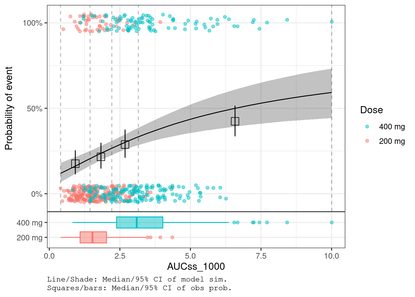

Figure 4.2

4.4 Model comparison

You can perform model comparison based on expected log pointwise predictive density (ELPD). ELPD is the Bayesian leave-one-out estimate (see ?loo-glossary).

Higher ELPD is better, therefore linear logistic regression model appears better than E_max model. However, elpd_diff is small and similar to se_diff (see here), therefore we can consider the difference to be not meaningful.

loo_bin_emax_hgly2 <- loo(ermod_bin_emax_hgly2)
loo_bin_hgly2 <- loo(ermod_bin_hgly2)

loo_compare(list(bin_emax_hgly2 = loo_bin_emax_hgly2, bin_hgly2 = loo_bin_hgly2))

               elpd_diff se_diff
bin_hgly2       0.0       0.0   
bin_emax_hgly2 -1.7       1.7   

Sometimes, loo() shows warnings on Pareto k estimates, which indicates problems in approximation of ELPD. Starting from BayesERtools 0.2.2, ELPD can also be evaluated with k-fold cross-validation. While it tends to be slower than loo (especially the E_max models), this will not face the challenge on approximation as written above.

set.seed(1234)

kfold_bin_emax_hgly2 <- kfold(ermod_bin_emax_hgly2)
kfold_bin_hgly2 <- kfold(ermod_bin_hgly2)

cmp_bin_kfold <- loo_compare(list(bin_emax_hgly2 = kfold_bin_emax_hgly2, bin_hgly2 = kfold_bin_hgly2))

cmp_bin_kfold

               elpd_diff se_diff
bin_hgly2       0.0       0.0   
bin_emax_hgly2 -0.9       2.2