8 Model diagnostics & comparison

This page showcase the model diagnosis and comparison for the E_max model

Show the code

library(tidyverse)
library(BayesERtools)
library(posterior)
library(tidybayes)
library(bayesplot)
library(loo)
library(here)
library(gt)

theme_set(theme_bw(base_size = 12))

8.1 Load data

Show the code

d_sim_emax

# A tibble: 300 × 9
    dose exposure response_1 response_2 cnt_a cnt_b cnt_c bin_d bin_e
                        
 1   100    4151.       12.8          1  5.71  2.33  7.83     0     1
 2   100    8067.       14.6          1  4.92  4.66  6.74     1     1
 3   100    4878.       12.8          1  4.88  4.21  4.68     1     1
 4   100    9713.       16.6          1  8.42  6.56  1.29     0     1
 5   100   11491.       14.4          0  4.37  3.96  3.55     0     1
 6   100    2452.       12.6          1  8.69  7.60  3.64     0     0
 7   100    5652.       14.8          1  6.61  3.95  5.13     0     0
 8   100    9939.       15.2          1  5.35  7.77  8.29     0     1
 9   100    5817.       14.6          0  5.61  2.24  9.60     0     1
10   100    5176.       13.7          1  6.06  1.79  8.74     0     1
# ℹ 290 more rows

8.2 Fit models

Sigmoidal E_max model
Regular E_max (γ fixed at 1)

Show the code

set.seed(1234)

ermod_sigemax <- dev_ermod_emax(
  data = d_sim_emax,
  var_resp = "response_1",
  var_exposure = "exposure",
  gamma_fix = NULL
)

ermod_sigemax


── Emax model ──────────────────────────────────────────────────────────────────
ℹ Use `plot_er()` to visualize ER curve

── Developed model ──

---- Emax model fit with rstanemax ----
         mean se_mean      sd   2.5%     25%     50%     75%    97.5%   n_eff
emax    11.59    0.31    5.89   4.82    7.34   10.10   14.24    27.50  368.24
e0       6.68    0.20    4.08  -3.67    4.78    7.68    9.71    11.48  436.14
ec50  5254.72  193.00 4475.71 801.17 2974.18 4673.97 6385.68 15736.00  537.81
gamma    1.06    0.02    0.50   0.32    0.70    0.97    1.33     2.26  543.20
sigma    1.27    0.00    0.05   1.18    1.24    1.27    1.31     1.39 1375.87
      Rhat
emax  1.01
e0    1.01
ec50  1.00
gamma 1.01
sigma 1.00
* Use `extract_stanfit()` function to extract raw stanfit object
* Use `extract_param()` function to extract posterior draws of key parameters
* Use `plot()` function to visualize model fit
* Use `posterior_predict()` or `posterior_predict_quantile()` function to get
  raw predictions or make predictions on new data
* Use `extract_obs_mod_frame()` function to extract raw data 
  in a processed format (useful for plotting)

Another model without sigmoidal component; will be used when we do model comparison.

Show the code

set.seed(1234)

ermod_emax <- dev_ermod_emax(
  data = d_sim_emax,
  var_resp = "response_1",
  var_exposure = "exposure",
  gamma_fix = 1
)

ermod_emax


── Emax model ──────────────────────────────────────────────────────────────────
ℹ Use `plot_er()` to visualize ER curve

── Developed model ──

---- Emax model fit with rstanemax ----
         mean se_mean      sd    2.5%     25%     50%     75%   97.5%   n_eff
emax    10.11    0.07    1.71    7.93    8.98    9.72   10.81   14.42  564.00
e0       7.32    0.08    2.00    2.41    6.41    7.66    8.70   10.13  572.38
ec50  4341.84   62.80 1871.39 1704.41 3062.61 3994.85 5323.78 9061.88  887.87
gamma    1.00     NaN    0.00    1.00    1.00    1.00    1.00    1.00     NaN
sigma    1.28    0.00    0.05    1.18    1.24    1.27    1.31    1.39 1440.04
      Rhat
emax  1.01
e0    1.01
ec50  1.00
gamma  NaN
sigma 1.00
* Use `extract_stanfit()` function to extract raw stanfit object
* Use `extract_param()` function to extract posterior draws of key parameters
* Use `plot()` function to visualize model fit
* Use `posterior_predict()` or `posterior_predict_quantile()` function to get
  raw predictions or make predictions on new data
* Use `extract_obs_mod_frame()` function to extract raw data 
  in a processed format (useful for plotting)

Show the code

d_draws_sigemax_summary <-
  summarize_draws(ermod_sigemax)

d_draws_sigemax_summary |>
  gt() |>
  fmt_number(decimals = 2)


```{=html}






variable
mean
median
sd
mad
q5
q95
rhat
ess_bulk
ess_tail




ec50
5,254.72
4,673.97
4,475.71
2,534.11
1,125.57
9,837.30
1.01
614.40
541.30


sigma
1.27
1.27
0.05
0.05
1.19
1.36
1.00
1,379.24
1,505.63


gamma
1.06
0.97
0.50
0.45
0.40
2.04
1.01
459.99
555.58


e0
6.68
7.68
4.08
3.42
−1.45
11.20
1.01
480.68
788.66


emax
11.59
10.10
5.89
4.79
5.20
23.06
1.01
429.41
533.51





```

variable	mean	median	sd	mad	q5	q95	rhat	ess_bulk	ess_tail
ec50	5,254.72	4,673.97	4,475.71	2,534.11	1,125.57	9,837.30	1.01	614.40	541.30
sigma	1.27	1.27	0.05	0.05	1.19	1.36	1.00	1,379.24	1,505.63
gamma	1.06	0.97	0.50	0.45	0.40	2.04	1.01	459.99	555.58
e0	6.68	7.68	4.08	3.42	−1.45	11.20	1.01	480.68	788.66
emax	11.59	10.10	5.89	4.79	5.20	23.06	1.01	429.41	533.51

Here is the example of highest-density continuous interval (HDCI) for the median of ED50. See here for more details.

Show the code

# HDCI of median.ED50
as_draws_df(ermod_sigemax) |>
  tidybayes::spread_rvars(ec50) |>
  tidybayes::median_hdci()

# A tibble: 1 × 6
   ec50 .lower .upper .width .point .interval
               
1 4674.   251.  9974.   0.95 median hdci

8.4 Fitted values

Fitted values without residual errors (i.e. PRED in NONMEM term) can be extracted with sim_er() function. .epred is the expected value prediction. See ?sim_er for detail.

Show the code

sim_er(ermod_sigemax) |> head()

# A tibble: 6 × 16
# Groups:   dose, exposure, response_1, response_2, cnt_a, cnt_b, cnt_c, bin_d,
#   bin_e, .row [1]
   dose exposure response_1 response_2 cnt_a cnt_b cnt_c bin_d bin_e  .row
                        
1   100    4151.       12.8          1  5.71  2.33  7.83     0     1     1
2   100    4151.       12.8          1  5.71  2.33  7.83     0     1     1
3   100    4151.       12.8          1  5.71  2.33  7.83     0     1     1
4   100    4151.       12.8          1  5.71  2.33  7.83     0     1     1
5   100    4151.       12.8          1  5.71  2.33  7.83     0     1     1
6   100    4151.       12.8          1  5.71  2.33  7.83     0     1     1
# ℹ 6 more variables: .chain , .iteration , .draw ,
#   .epred , .linpred , .prediction

You can specify output_type = "median_qi" to get median and quantile intervals of the prediction.

Show the code

ersim_sigemax_med_qi <-
  sim_er(ermod_sigemax, output_type = "median_qi")

ersim_sigemax_med_qi |>
  arrange(.row) |>
  head() |>
  gt(rownames_to_stub = TRUE) |>
  fmt_number(decimals = 2, columns = -.row)


```{=html}







dose
exposure
response_1
response_2
cnt_a
cnt_b
cnt_c
bin_d
bin_e
.row
.epred
.epred.lower
.epred.upper
.linpred
.linpred.lower
.linpred.upper
.prediction
.prediction.lower
.prediction.upper
.width
.point
.interval




1
100.00
4,151.15
12.80
1.00
5.71
2.33
7.83
0.00
1.00
1
12.62
12.33
12.92
12.62
12.33
12.92
12.63
10.03
15.29
0.95
median
qi


2
100.00
8,067.26
14.58
1.00
4.92
4.66
6.74
1.00
1.00
2
14.14
13.93
14.35
14.14
13.93
14.35
14.14
11.69
16.69
0.95
median
qi


3
100.00
4,877.67
12.76
1.00
4.88
4.21
4.68
1.00
1.00
3
13.00
12.73
13.24
13.00
12.73
13.24
12.98
10.52
15.51
0.95
median
qi


4
100.00
9,712.93
16.55
1.00
8.42
6.56
1.29
0.00
1.00
4
14.53
14.31
14.74
14.53
14.31
14.74
14.51
12.07
17.07
0.95
median
qi


5
100.00
11,490.74
14.41
0.00
4.37
3.96
3.55
0.00
1.00
5
14.86
14.64
15.08
14.86
14.64
15.08
14.87
12.36
17.37
0.95
median
qi


6
100.00
2,451.55
12.60
1.00
8.69
7.60
3.64
0.00
0.00
6
11.48
10.87
12.07
11.48
10.87
12.07
11.47
8.86
14.00
0.95
median
qi





```

8.5 Diagnostic plots

We use the bayesplot package (Cheat sheet) to visualize the model fit.

8.5.1 Convergence

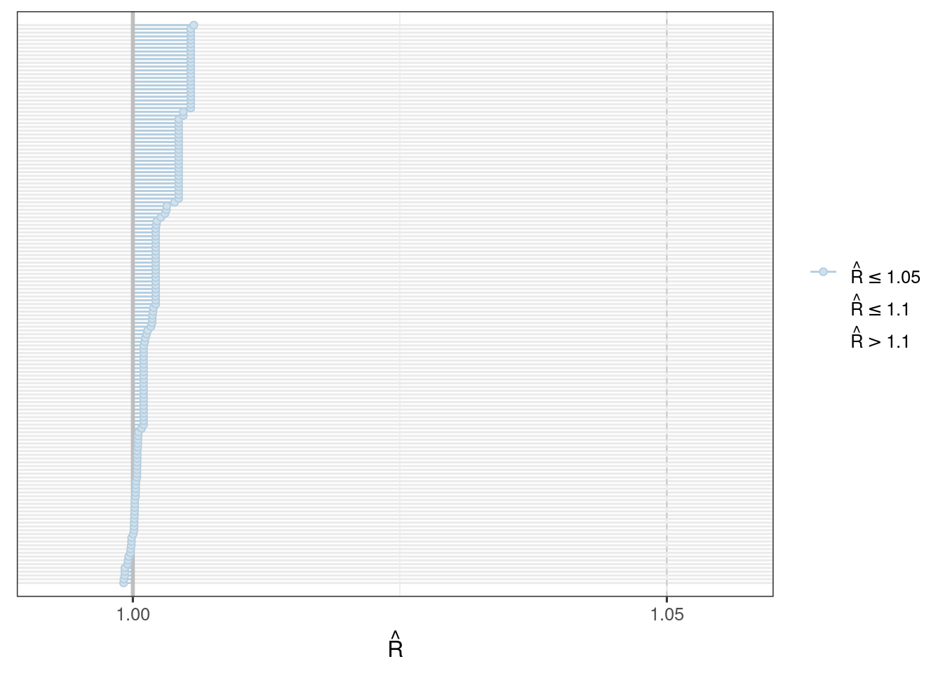
Good fit results in:

Parameter distributions from MCMC chains should overlap
Trace plots should not show any trend
Rhat close to 1 (e.g. < 1.1)

Show the code

d_draws_sigemax <- as_draws_df(ermod_sigemax)
mcmc_dens_overlay(d_draws_sigemax)
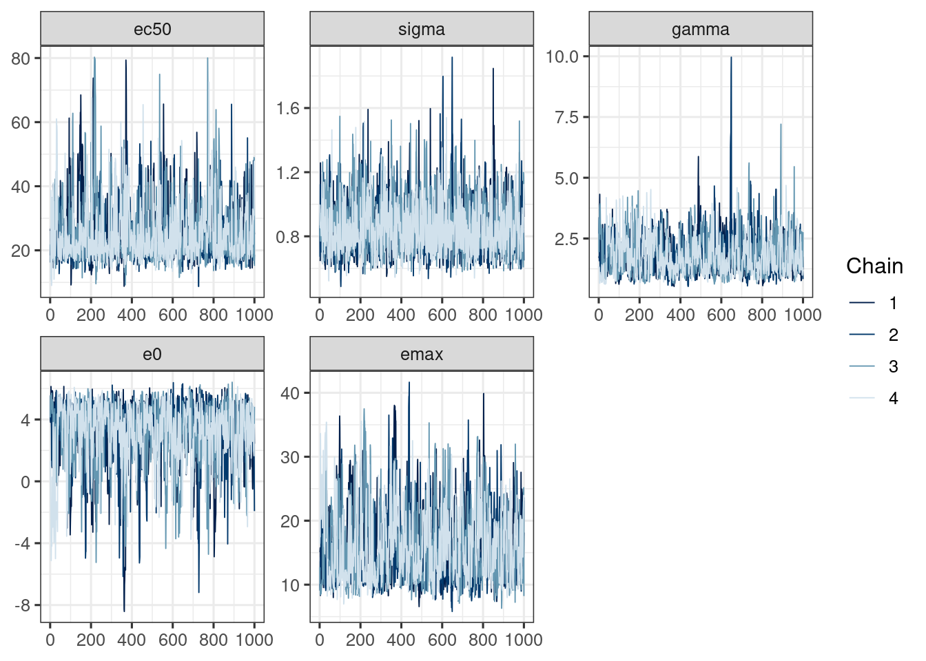
mcmc_trace(d_draws_sigemax)
mcmc_rhat(rhat(ermod_sigemax$mod$stanfit))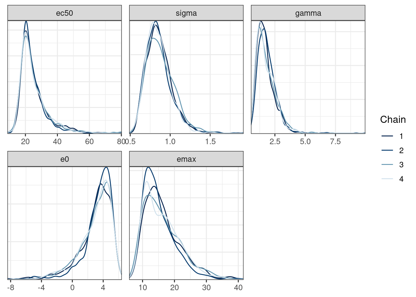

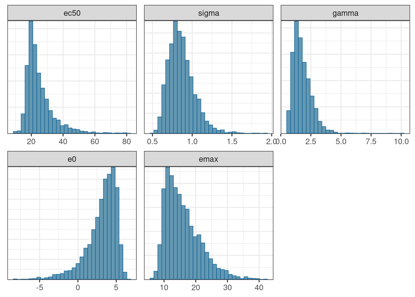
8.5.2 Parameter estimates distribution

mcmc_hist
Parameter covariance

Show the code

mcmc_hist(d_draws_sigemax)

`stat_bin()` using `bins = 30`. Pick better value with `binwidth`.

Show the code

mcmc_pairs(d_draws_sigemax,
  off_diag_args = list(size = 0.5, alpha = 0.25))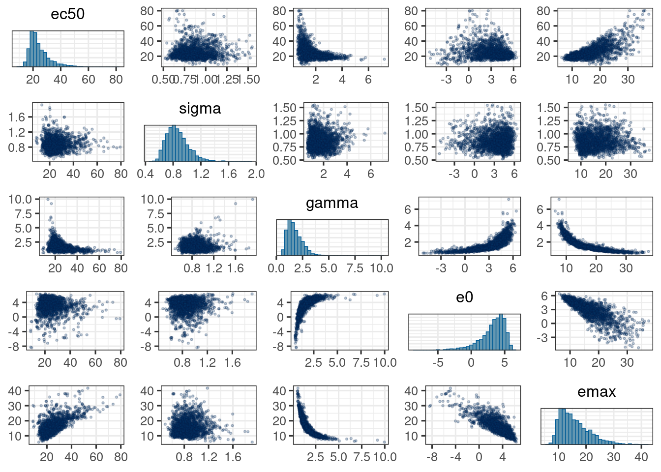

8.5.3 GOF plots

Show the code

plot_er(ermod_sigemax, show_orig_data = TRUE)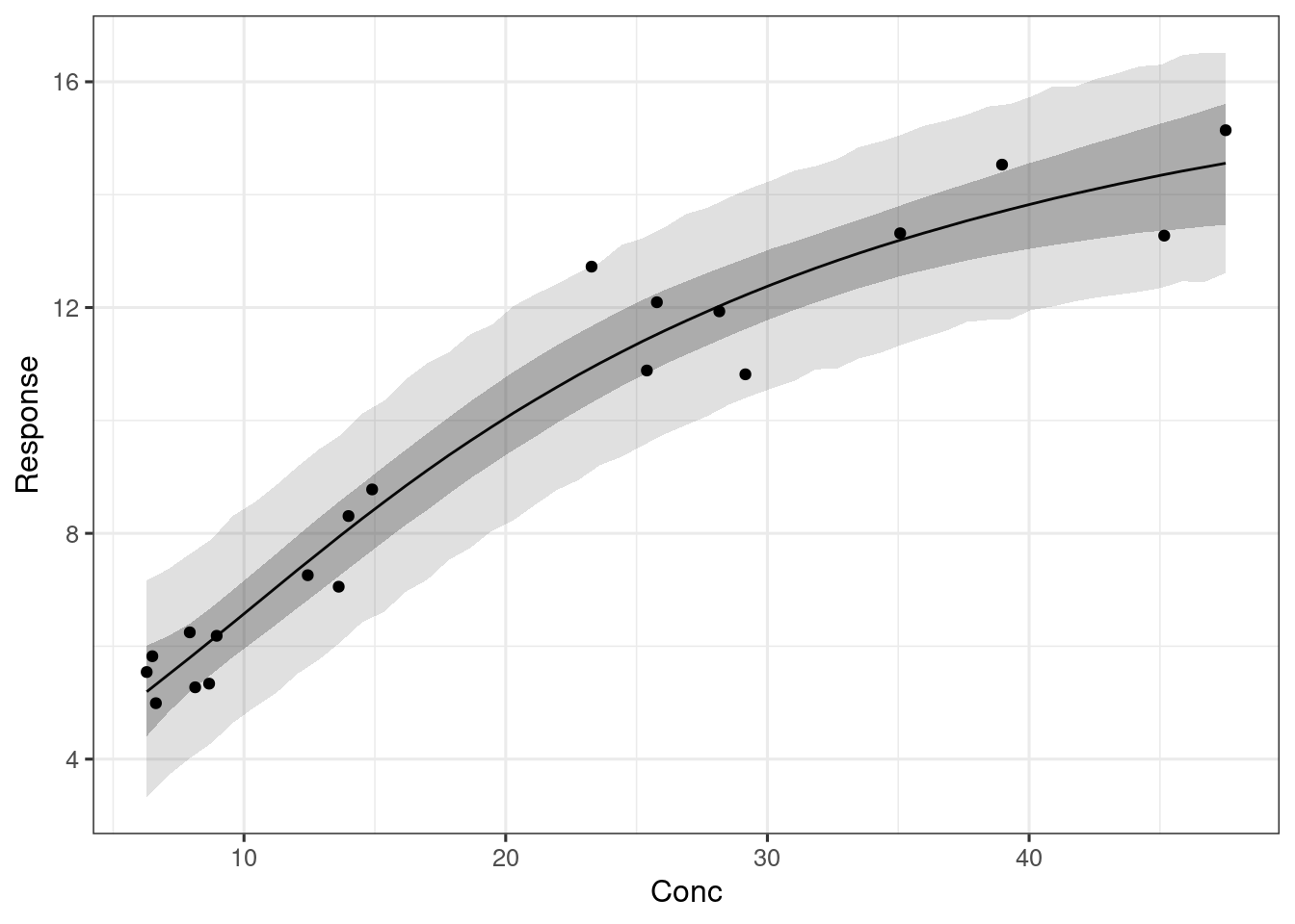

Show the code

# Preparation for diagnostic plots
ersim_sigemax_med_qi <- sim_er(ermod_sigemax, output_type = "median_qi")

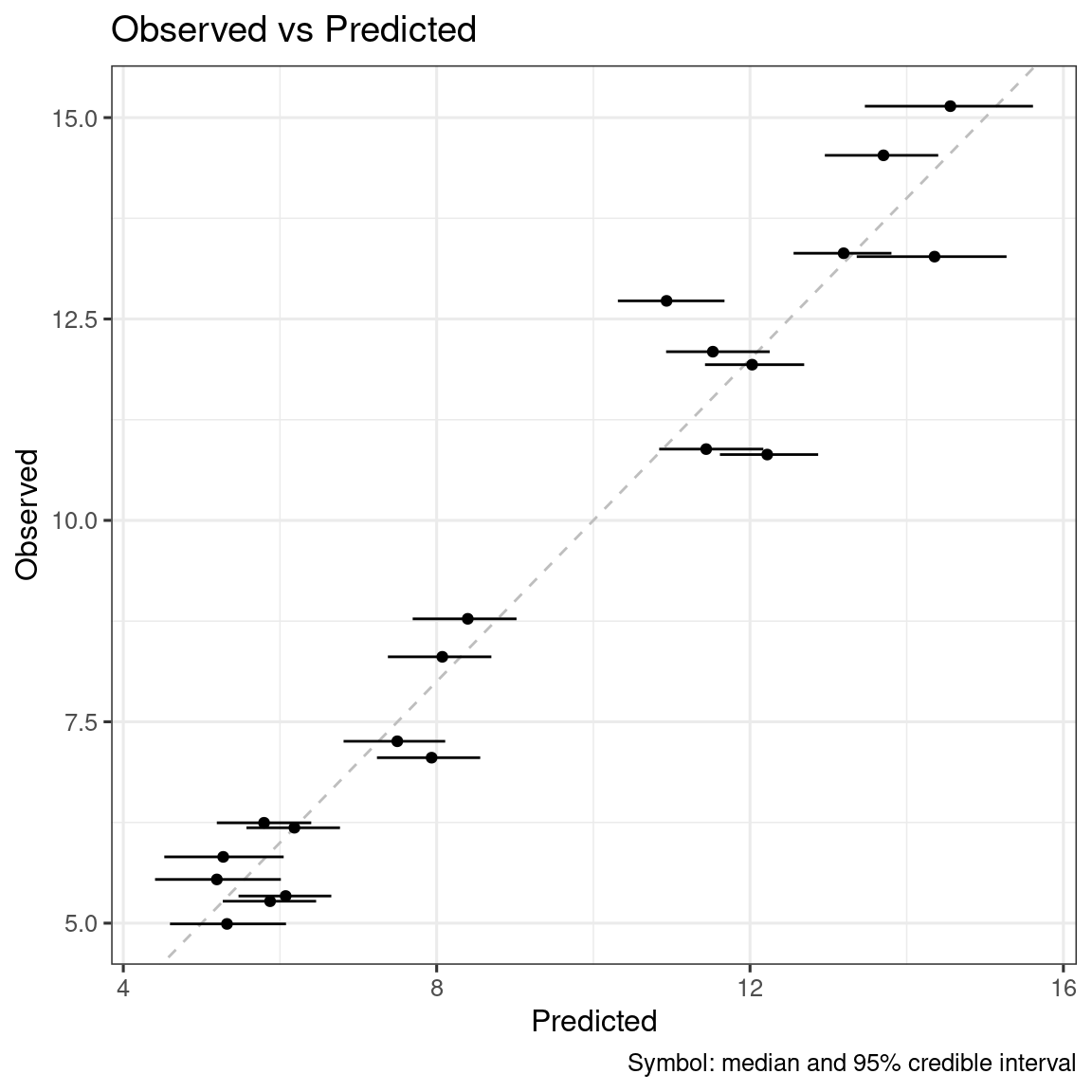
ersim_sigemax_med_qi |>
  ggplot(aes(x = .epred, y = response_1)) +
  geom_abline(linetype = 2, color = "grey") +
  geom_point() +
  geom_errorbarh(aes(xmin = .epred.lower, xmax = .epred.upper), height = 0) +
  labs(title = "Observed vs Predicted",
    x = "Predicted",
    y = "Observed",
    caption = "Symbol: median and 95% credible interval")

Show the code

ersim_sigemax_w_resid <-
  sim_er(ermod_sigemax) |>
  mutate(.residual = response_1 - .epred) # Add residuals for plotting
ersim_sigemax_w_resid_med_qi <- median_qi(ersim_sigemax_w_resid)

ersim_sigemax_w_resid_med_qi |>
  ggplot(aes(x = .epred, y = .residual)) +
  xlab("Predicted (linear)") +
  ylab("Residuals") +
  geom_point() +
  geom_errorbar(aes(ymin = .residual.lower, ymax = .residual.upper), width = 0) +
  geom_hline(aes(yintercept = 2), lty = 2, colour = "grey70") +
  geom_hline(aes(yintercept = -2), lty = 2, colour = "grey70")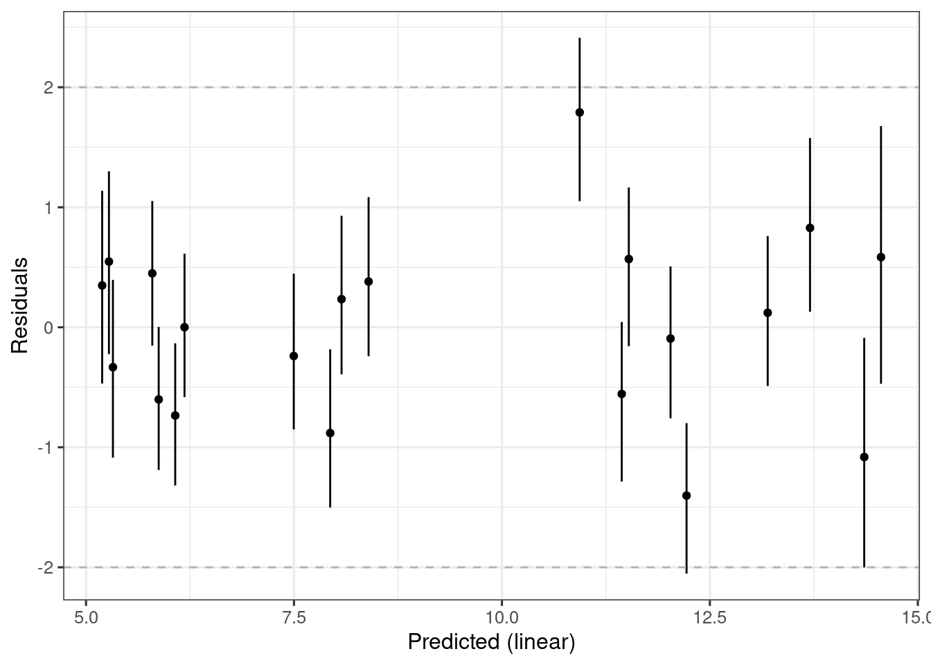

Show the code

ersim_sigemax_w_resid_med_qi |>
  ggplot(aes(sample = .residual)) +
  geom_qq() +
  geom_qq_line(colour = "steelblue", lty = 2, alpha = 0.4) +
  coord_equal() +
  xlab("Theoretical") +
  ylab("Sample")

8.6 Model comparison

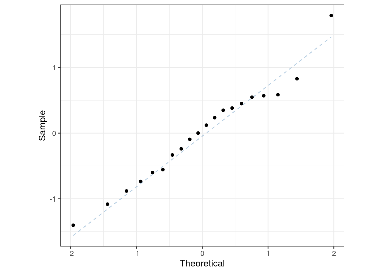
You can perform model comparison based on expected log pointwise predictive density (ELPD). ELPD is the Bayesian leave-one-out estimate (see ?loo-glossary).

Higher ELPD is better, therefore E_max model with γ fixed to be 1 appears better. However, elpd_diff is tiny and smaller than se_diff (see here), therefore we can consider the difference to be not meaningful.

Show the code

loo_sigemax <- loo(ermod_sigemax)
loo_emax <- loo(ermod_emax)

loo_compare(list(sigemax = loo_sigemax, emax = loo_emax))

        elpd_diff se_diff
emax     0.0       0.0   
sigemax -0.9       0.4