Show the code
library(tidyverse)
library(BayesERtools)
library(here)
library(posterior)
library(bayesplot)
library(gt)

theme_set(theme_bw(base_size = 12))This page showcase the model diagnosis and performance evaluation on the ER model for binary endpoint.
library(tidyverse)
library(BayesERtools)
library(here)
library(posterior)
library(bayesplot)
library(gt)
theme_set(theme_bw(base_size = 12))data(d_sim_binom_cov)
d_sim_binom_cov_2 <-
d_sim_binom_cov |>
mutate(
AUCss_1000 = AUCss / 1000, BAGE_10 = BAGE / 10,
BWT_10 = BWT / 10, BHBA1C_5 = BHBA1C / 5,
Dose = glue::glue("{Dose_mg} mg")
)
# Grade 2+ hypoglycemia
df_er_ae_hgly2 <- d_sim_binom_cov_2 |> filter(AETYPE == "hgly2")
# Grade 2+ diarrhea
df_er_ae_dr2 <- d_sim_binom_cov_2 |> filter(AETYPE == "dr2")
var_resp <- "AEFLAG"
var_exposure <- "AUCss_1000"There is clear trend of E-R for hyperglycemia (95% CI doesn’t include 0) while the evidence of E-R is not seen for diarrhea (95% CI includes 0).
set.seed(1234)
ermod_bin_hgly2 <- dev_ermod_bin(
  data = df_er_ae_hgly2,
  var_resp = var_resp,
  var_exposure = var_exposure
)
plot_er_gof(ermod_bin_hgly2, var_group = "Dose", show_coef_exp = TRUE)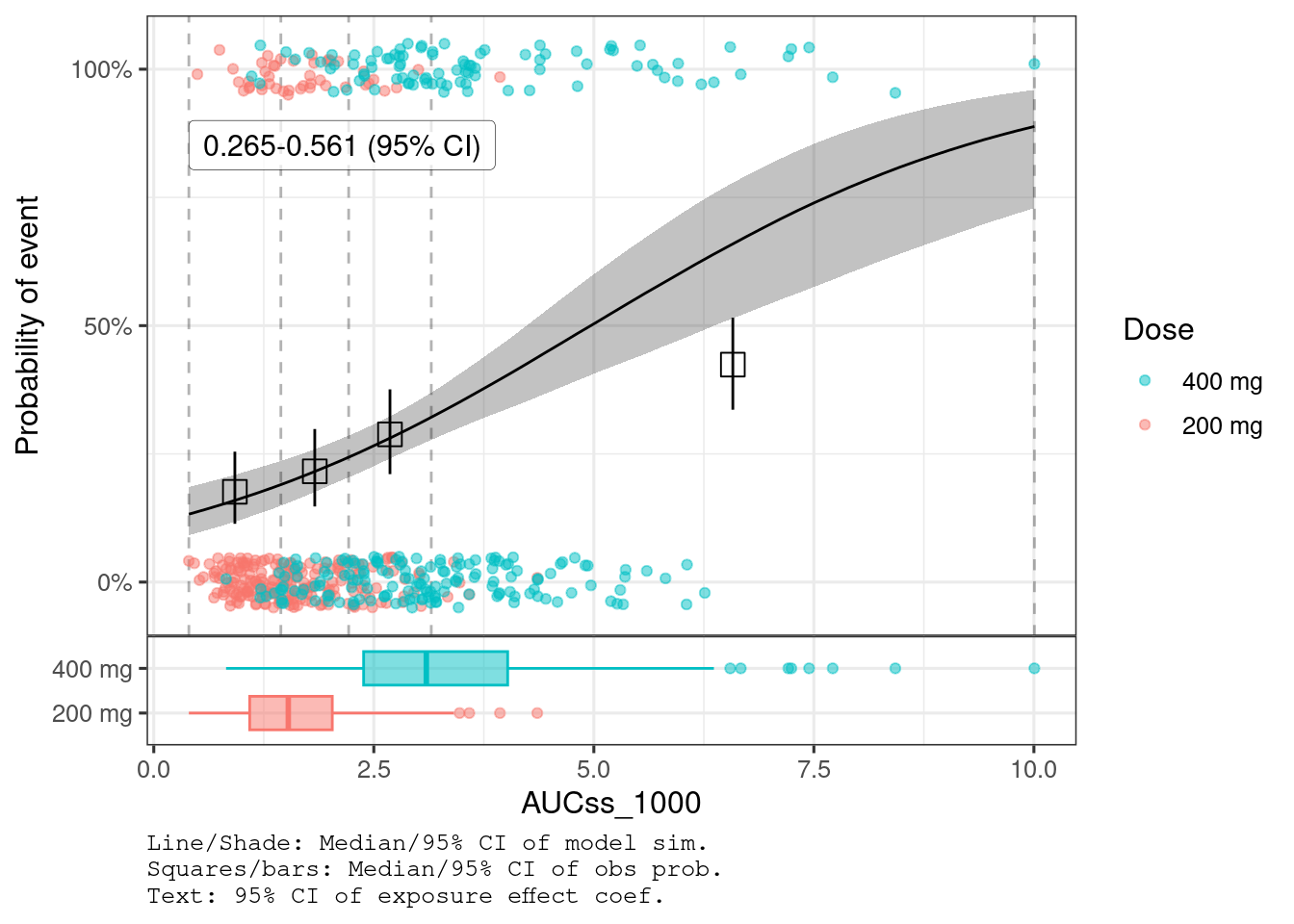
set.seed(1234)
ermod_bin_dr2 <- dev_ermod_bin(
  data = df_er_ae_dr2,
  var_resp = var_resp,
  var_exposure = var_exposure
)
plot_er_gof(ermod_bin_dr2, var_group = "Dose", show_coef_exp = TRUE)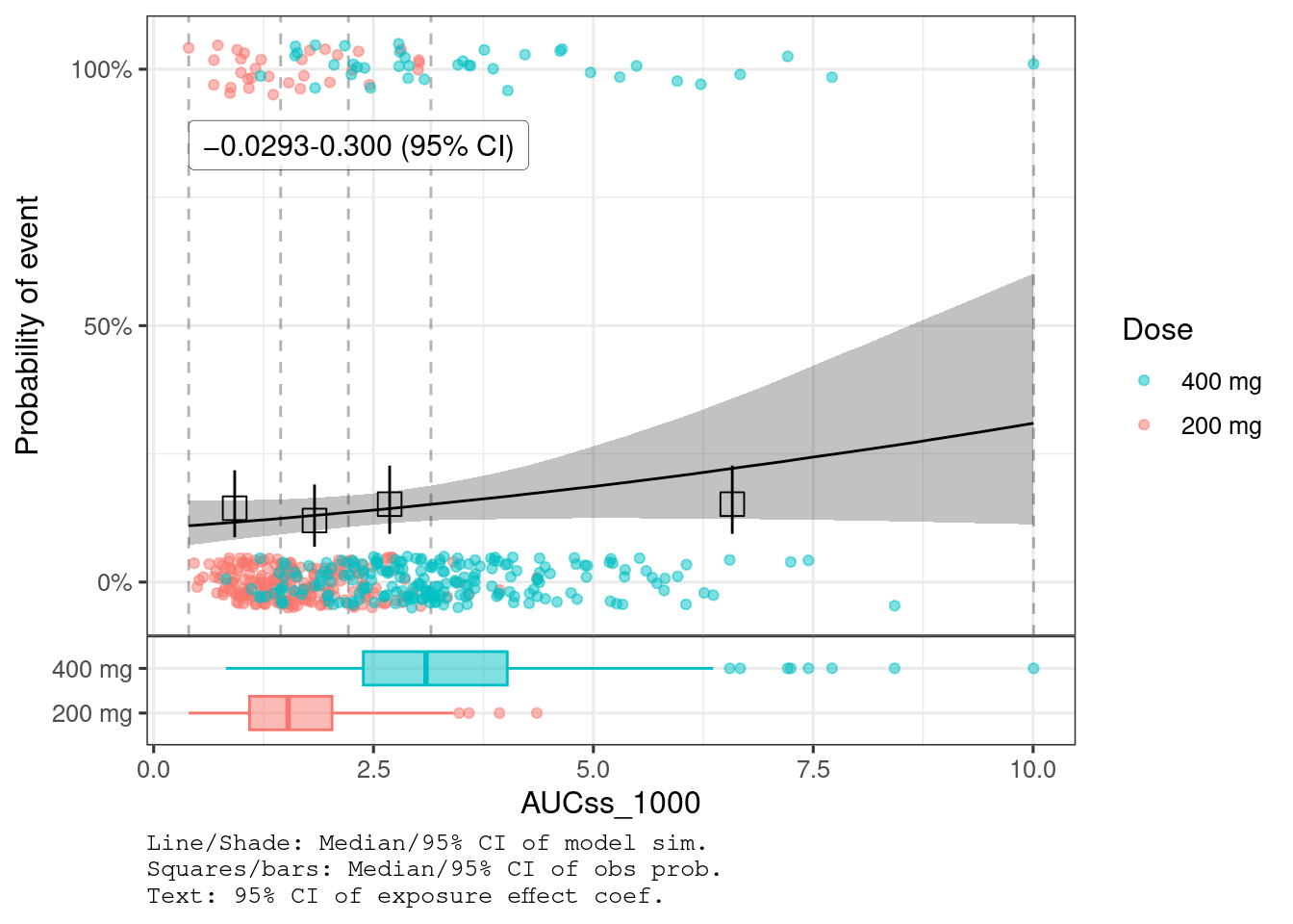
You can see that AUCss effect is much stronger for hyperglycemia than diarrhea.
ermod_bin_hgly2 |>
  summarize_draws(mean, median, sd, ~ quantile2(.x, probs = c(0.025, 0.975)),
    default_convergence_measures()) |>
  gt() |>
fmt_number(n_sigfig = 3)| variable | mean | median | sd | q2.5 | q97.5 | rhat | ess_bulk | ess_tail |
|---|---|---|---|---|---|---|---|---|
| (Intercept) | −2.05 | −2.04 | 0.234 | −2.51 | −1.59 | 1.00 | 2,230 | 1,870 |
| AUCss_1000 | 0.412 | 0.412 | 0.0761 | 0.265 | 0.561 | 1.00 | 2,150 | 2,140 |
ermod_bin_dr2 |>
  summarize_draws(mean, median, sd, ~ quantile2(.x, probs = c(0.025, 0.975)),
    default_convergence_measures()) |>
  gt() |>
fmt_number(n_sigfig = 3)| variable | mean | median | sd | q2.5 | q97.5 | rhat | ess_bulk | ess_tail |
|---|---|---|---|---|---|---|---|---|
| (Intercept) | −2.15 | −2.15 | 0.255 | −2.65 | −1.67 | 1.00 | 2,830 | 2,320 |
| AUCss_1000 | 0.135 | 0.134 | 0.0832 | −0.0293 | 0.300 | 1.00 | 2,810 | 2,570 |
We can calculate predictive performance metrics such as AUC-ROC with eval_ermod() function. Options for evaluation data are:
eval_type = "training": training dataeval_type = "test": test data (supply to newdata argument)eval_type = "kfold": k-fold cross-validationmetrics_hgly2_train <- eval_ermod(ermod_bin_hgly2, eval_type = "training")
metrics_hgly2_kfold <- eval_ermod(ermod_bin_hgly2, eval_type = "kfold")metrics_hgly2_train |>
gt() |>
fmt_number(n_sigfig = 3)| .metric | .estimator | .estimate |
|---|---|---|
| roc_auc | binary | 0.650 |
| mn_log_loss | binary | 0.555 |
metrics_hgly2_kfold |>
  gt() |>
  fmt_number(n_sigfig = 3) |>
fmt_integer(columns = c("fold_id"))| fold_id | .metric | .estimator | .estimate |
|---|---|---|---|
| 1 | roc_auc | binary | 0.631 |
| 2 | roc_auc | binary | 0.607 |
| 3 | roc_auc | binary | 0.684 |
| 4 | roc_auc | binary | 0.670 |
| 5 | roc_auc | binary | 0.663 |
| 1 | mn_log_loss | binary | 0.602 |
| 2 | mn_log_loss | binary | 0.572 |
| 3 | mn_log_loss | binary | 0.534 |
| 4 | mn_log_loss | binary | 0.581 |
| 5 | mn_log_loss | binary | 0.500 |
Although credible intervals are preferred, there is a concept called the probability of direction which is somewhat similar to the p-value, in which the probability of the effect being far from NULL (usually set to 0) is calculated.
See ?p_direction and vignette for detail.
The exposure effect is so clear that none of the MCMC sample is below 0, leading to a “p-value” of 0. Since there were 4000 MCMC samples (nrow(as_draws_df(ermod_bin_hgly2))), it is expected that the p-value is less than 1/4000 * 2, i.e. < 0.0005 (multiplication with 2 corresponds to two-sided test).
bayestestR::p_direction(ermod_bin_hgly2, as_p = TRUE, as_num = TRUE)[1] 0
1 / length(as_draws(ermod_bin_hgly2)$AUCss_1000) * 2[1] 5e-04
bayestestR::p_direction(ermod_bin_dr2, as_p = TRUE, as_num = TRUE)[1] 0.108
# Below is a direct calculation of this value
mean(as_draws(ermod_bin_dr2)$AUCss_1000 < 0) * 2
[1] 0.108
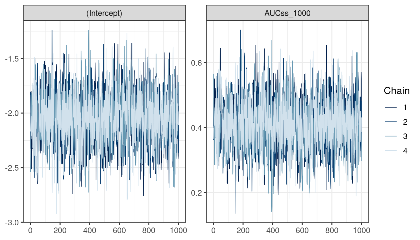
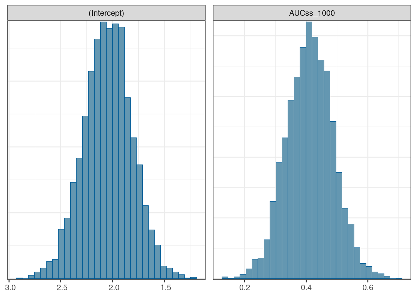
We use the bayesplot package (Cheat sheet) to visualize the model fit.
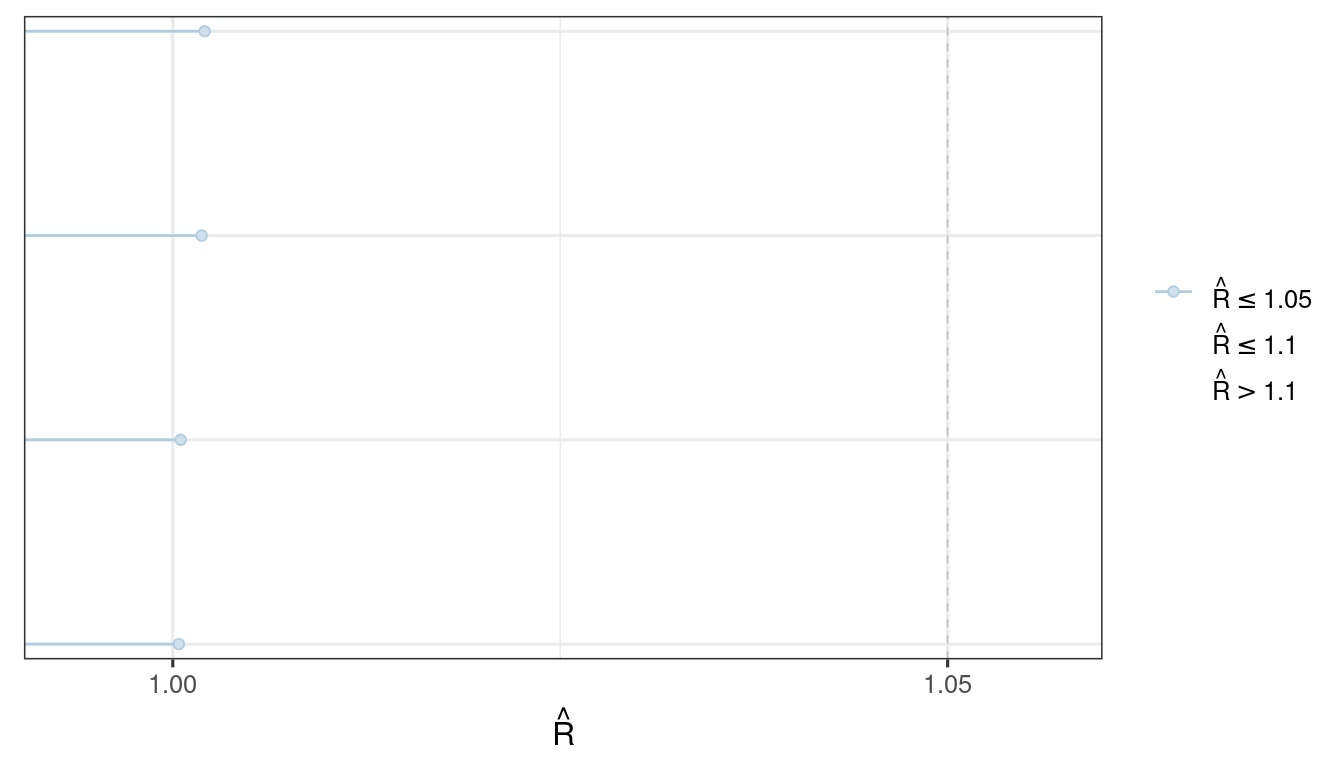
Good fit results in:
Rhat close to 1 (e.g. < 1.1)d_draws_bin_hgly2 <- as_draws_df(ermod_bin_hgly2)
mcmc_dens_overlay(d_draws_bin_hgly2)
mcmc_trace(d_draws_bin_hgly2)
mcmc_rhat(rhat(ermod_bin_hgly2$mod$stanfit))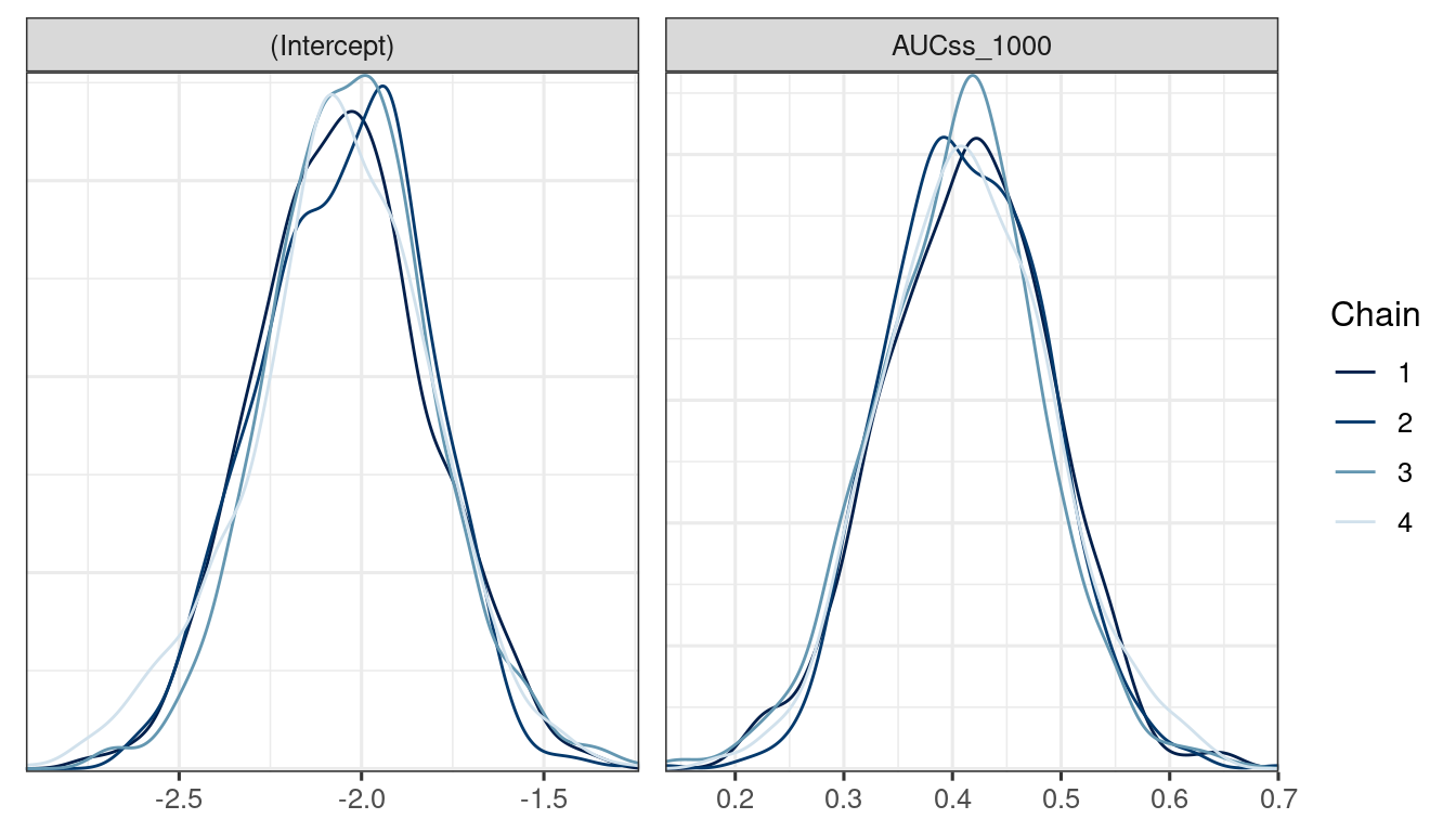
mcmc_hist(d_draws_bin_hgly2)`stat_bin()` using `bins = 30`. Pick better value `binwidth`.
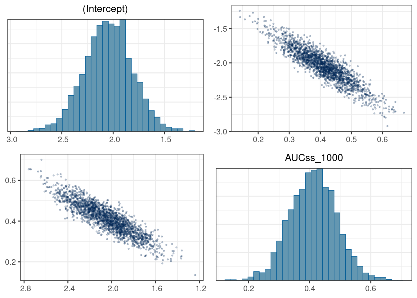
mcmc_pairs(d_draws_bin_hgly2,
  off_diag_args = list(size = 0.5, alpha = 0.25))