Show the code
library(tidyverse)
library(BayesERtools)
library(posterior)
library(bayesplot)
library(loo)
library(here)
library(gt)

theme_set(theme_bw(base_size = 12))This page showcase the model simulation using the Emax model with no covariate.
library(tidyverse)
library(BayesERtools)
library(posterior)
library(bayesplot)
library(loo)
library(here)
library(gt)
theme_set(theme_bw(base_size = 12))d_sim_emax# A tibble: 300 × 9
dose exposure response_1 response_2 cnt_a cnt_b cnt_c bin_d bin_e
set.seed(1234)

ermod_sigemax <- dev_ermod_emax(
  data = d_sim_emax,
  var_resp = "response_1",
  var_exposure = "exposure",
  gamma_fix = NULL
)

ermod_sigemax
── Emax model ──────────────────────────────────────────────────────────────────
ℹ Use `plot_er()` to visualize ER curve

── Developed model ──

---- Emax model fit with rstanemax ----
         mean se_mean      sd   2.5%     25%     50%     75%    97.5%   n_eff
emax    11.70    0.29    5.84   4.65    7.35   10.19   14.52    27.20  414.18
e0       6.45    0.21    4.40  -5.11    4.58    7.58    9.63    11.59  436.99
ec50  4892.89  129.05 3858.03 649.97 2787.66 4537.64 6219.22 12022.48  893.78
gamma    1.07    0.02    0.51   0.34    0.70    0.96    1.34     2.32  575.85
sigma    1.27    0.00    0.05   1.18    1.24    1.27    1.31     1.38 1513.21
      Rhat
emax  1.01
e0    1.01
ec50  1.00
gamma 1.01
sigma 1.00
* Use `extract_stanfit()` function to extract raw stanfit object
* Use `extract_param()` function to extract posterior draws of key parameters
* Use `plot()` function to visualize model fit
* Use `posterior_predict()` or `posterior_predict_quantile()` function to get
  raw predictions or make predictions on new data
* Use `extract_obs_mod_frame()` function to extract raw data
  in a processed format (useful for plotting)
Another model without sigmoidal component; will be used when we do model comparison.
set.seed(1234)

ermod_emax <- dev_ermod_emax(
  data = d_sim_emax,
  var_resp = "response_1",
  var_exposure = "exposure",
  gamma_fix = 1
)

ermod_emax
── Emax model ──────────────────────────────────────────────────────────────────
ℹ Use `plot_er()` to visualize ER curve

── Developed model ──

---- Emax model fit with rstanemax ----
         mean se_mean      sd    2.5%     25%     50%     75%   97.5%   n_eff
emax    10.17    0.06    1.66    7.96    9.02    9.79   10.96   14.39  704.66
e0       7.24    0.07    1.95    2.56    6.20    7.58    8.65    9.98  697.52
ec50  4213.96   57.75 1720.01 1743.37 2943.96 3917.32 5202.32 8117.56  887.11
gamma    1.00     NaN    0.00    1.00    1.00    1.00    1.00    1.00     NaN
sigma    1.27    0.00    0.05    1.17    1.24    1.27    1.31    1.39 1246.77
      Rhat
emax  1.01
e0    1.01
ec50  1.01
gamma  NaN
sigma 1.00
* Use `extract_stanfit()` function to extract raw stanfit object
* Use `extract_param()` function to extract posterior draws of key parameters
* Use `plot()` function to visualize model fit
* Use `posterior_predict()` or `posterior_predict_quantile()` function to get
  raw predictions or make predictions on new data
* Use `extract_obs_mod_frame()` function to extract raw data
  in a processed format (useful for plotting)
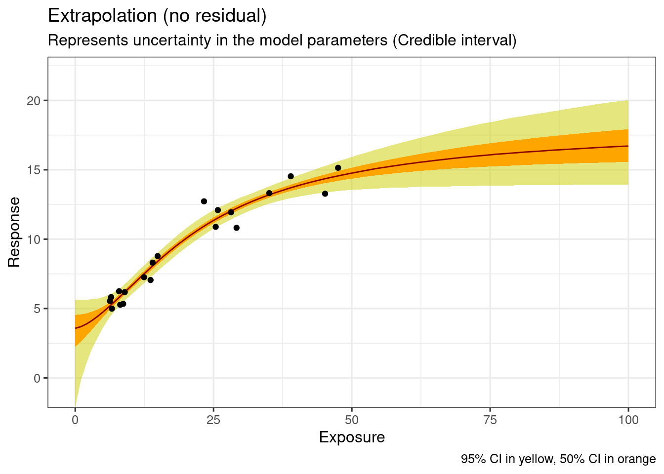
This represents uncertainty in the model parameters.
p(f(theta)|xnew, yobs)new_conc_vec <- seq(0, 70000, by = 500)
ersim_sigemax <-
sim_er_new_exp(ermod_sigemax, new_conc_vec)
ersim_sigemax_med_qi <-
ersim_sigemax |>
calc_ersim_med_qi(qi_width = c(0.5, 0.95))
ggplot(
data = ersim_sigemax_med_qi,
mapping = aes(x = exposure, y = .epred)
) +
geom_ribbon(
data = ersim_sigemax_med_qi |> filter(.width == 0.95),
mapping = aes(ymin = .epred.lower, ymax = .epred.upper),
fill = "yellow3",
alpha = 0.5
) +
geom_ribbon(
data = ersim_sigemax_med_qi |> filter(.width == 0.5),
mapping = aes(ymin = .epred.lower, ymax = .epred.upper),
fill = "orange1"
) +
geom_line(
data = ersim_sigemax_med_qi |> filter(.width == 0.5),
col = "darkred"
) +
geom_point(
data = d_sim_emax,
mapping = aes(y = response_1)
) +
coord_cartesian(ylim = c(5, 22)) +
labs(
x = "Exposure",
y = "Response",
title = "Extrapolation (no residual)",
subtitle = paste(
"Represents uncertainty in the model parameters",
"(Credible interval)"
),
caption = "95% CI in yellow, 50% CI in orange"
)
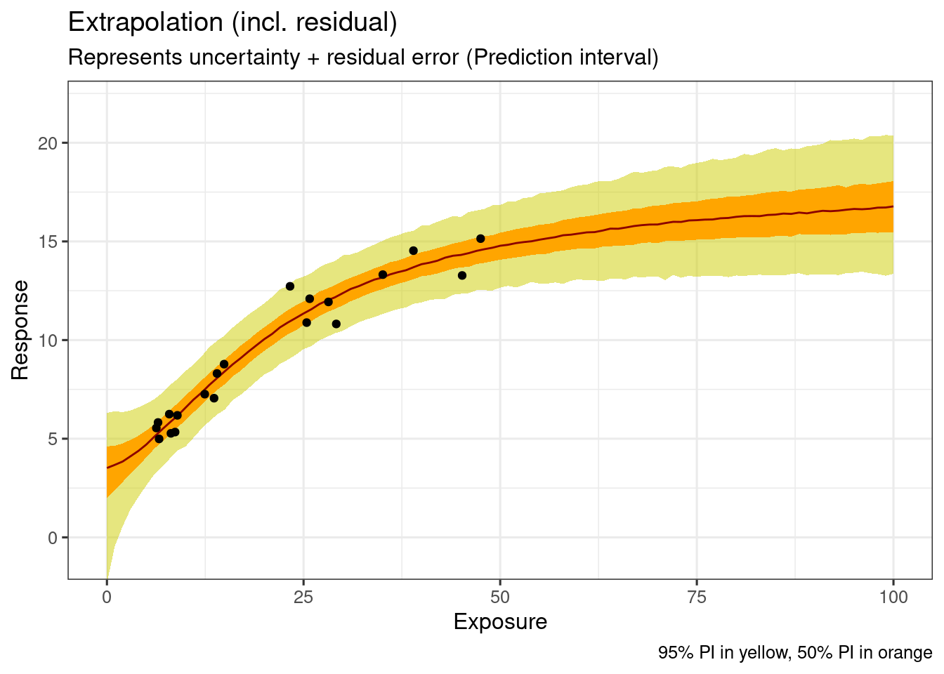
This represents uncertainty in the model parameters plus the residual error.
p(ynew|xnew, yobs)ggplot(
data = ersim_sigemax_med_qi,
mapping = aes(x = exposure, y = .prediction)
) +
geom_ribbon(
data = ersim_sigemax_med_qi |> filter(.width == 0.95),
mapping = aes(ymin = .prediction.lower, ymax = .prediction.upper),
fill = "yellow3",
alpha = 0.5
) +
geom_ribbon(
data = ersim_sigemax_med_qi |> filter(.width == 0.5),
mapping = aes(ymin = .prediction.lower, ymax = .prediction.upper),
fill = "orange1"
) +
geom_line(
data = ersim_sigemax_med_qi |> filter(.width == 0.5),
col = "darkred"
) +
geom_point(
data = d_sim_emax,
mapping = aes(y = response_1)
) +
coord_cartesian(ylim = c(5, 22)) +
labs(
x = "Exposure",
y = "Response",
title = "Extrapolation (incl. residual)",
subtitle = "Represents uncertainty + residual error (Prediction interval)",
caption = "95% PI in yellow, 50% PI in orange"
)
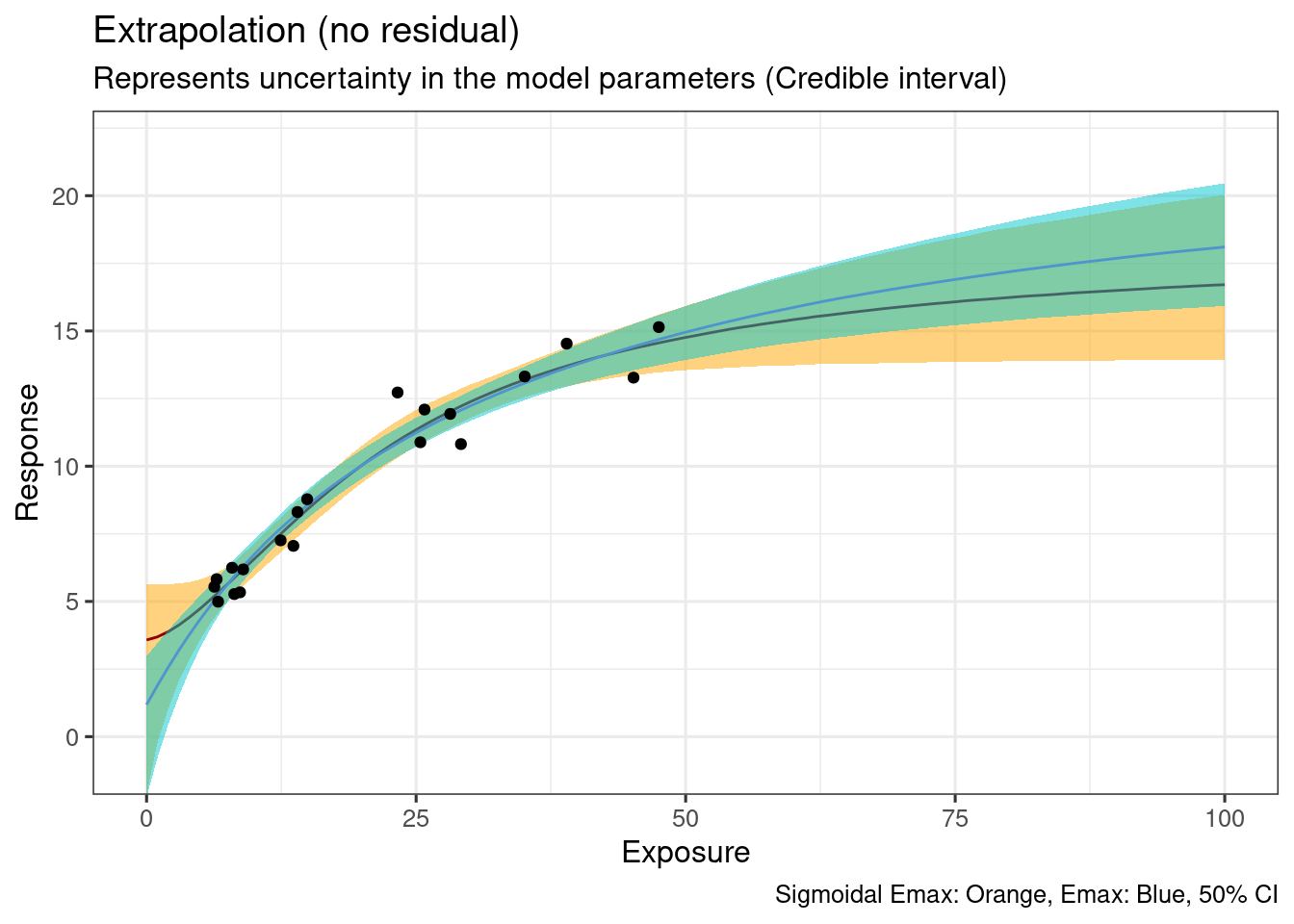
No discernible difference between the two models.
ersim_emax <-
  sim_er_new_exp(ermod_emax, new_conc_vec)

ersim_emax_med_qi <-
  ersim_emax |>
  calc_ersim_med_qi(qi_width = c(0.5, 0.95))

ggplot(
  data = ersim_sigemax_med_qi,
  mapping = aes(x = exposure, y = .epred)
) +
  geom_ribbon(
    data = ersim_sigemax_med_qi |> filter(.width == 0.95),
    mapping = aes(ymin = .epred.lower, ymax = .epred.upper),
    fill = "orange1",
    alpha = 0.5
  ) +
  geom_line(
    data = ersim_sigemax_med_qi |> filter(.width == 0.95),
    col = "darkred"
  ) +
  geom_ribbon(
    data = ersim_emax_med_qi |> filter(.width == 0.95),
    mapping = aes(ymin = .epred.lower, ymax = .epred.upper),
    fill = "turquoise3",
    alpha = 0.5
  ) +
  geom_line(
    data = ersim_emax_med_qi |> filter(.width == 0.95),
    col = "steelblue3"
  ) +
  geom_point(
    data = d_sim_emax,
    mapping = aes(y = response_1)
  ) +
  coord_cartesian(ylim = c(5, 22)) +
  labs(
    x = "Exposure",
    y = "Response",
    title = "Extrapolation (no residual)",
    subtitle = paste(
      "Represents uncertainty in the model parameters",
      "(Credible interval)"
    ),
    caption = "Sigmoidal Emax: Orange, Emax: Blue, 50% CI"
  )