Show the code
library(tidyverse)
library(here)

theme_set(theme_bw(base_size = 12))

set.seed(1234)This page shows examples of data generation for Emax model with and without covariates.
library(tidyverse)
library(here)
theme_set(theme_bw(base_size = 12))
set.seed(1234)n <- 20 # number of subjects
E0 <- 5 # effect at 0 concentration
Emax <- 10 # maximal effect
EC50 <- 20 # concentration at half maximal effect
h <- 2 # Hill coefficient
set.seed(130)
c.is <- 50 * runif(n) # exposure
set.seed(130)
eps <- rnorm(n) # residual error
y.is <- E0 + ((Emax * c.is^h) / (c.is^h + EC50^h)) + eps
d_example_emax_nocov <- tibble(Conc = c.is, Y = y.is)ggplot(d_example_emax_nocov, aes(Conc, Y)) +
geom_point() +
geom_smooth(formula = y ~ x, method = "loess", se = F, col = "darkgrey") +
scale_x_continuous("Exposure", breaks = c(3, 10, 30, 100))
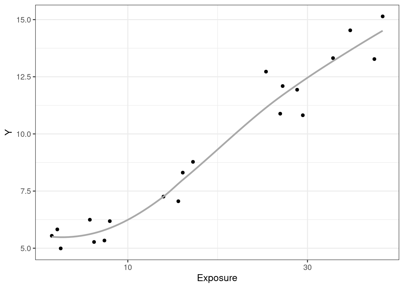
ggplot(d_example_emax_nocov, aes(Conc, Y)) +
geom_point() +
geom_smooth(formula = y ~ x, method = "loess", se = F, col = "darkgrey") +
scale_x_log10("Exposure", breaks = c(3, 10, 30, 100))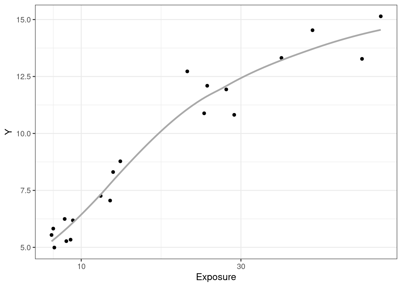
Only one covariate (Prognostic factor positive/negative)
Ngp <- 2
N <- 20 * Ngp
GPid <- as.factor(rep(c("A", "B"), each = 20))

# Set parameters
E0 <- 5
EC50 <- 15
h <- 2
beta1 <- .7

# Calc response
set.seed(12345)

d_example_emax_cov <-
  tibble(GP = GPid) |>
  mutate(
    c.is = 50 * runif(N), eps = rnorm(N)
  ) |>
  mutate(
    Emax.i = ifelse(GP == "A", 10, 15)
  ) |>
  mutate(y.is = E0 + ((Emax.i * c.is^h) / (c.is^h + EC50^h)) + eps) |>
mutate(Conc = c.is, Y = y.is)ggplot(d_example_emax_cov, aes(Conc, Y)) +
geom_point(aes(colour = GP)) +
geom_smooth(aes(group = GP, colour = GP), se = F) +
scale_x_continuous("Exposure") +
theme(legend.position = "top")`geom_smooth()` using method = 'loess' and formula = 'y ~ x'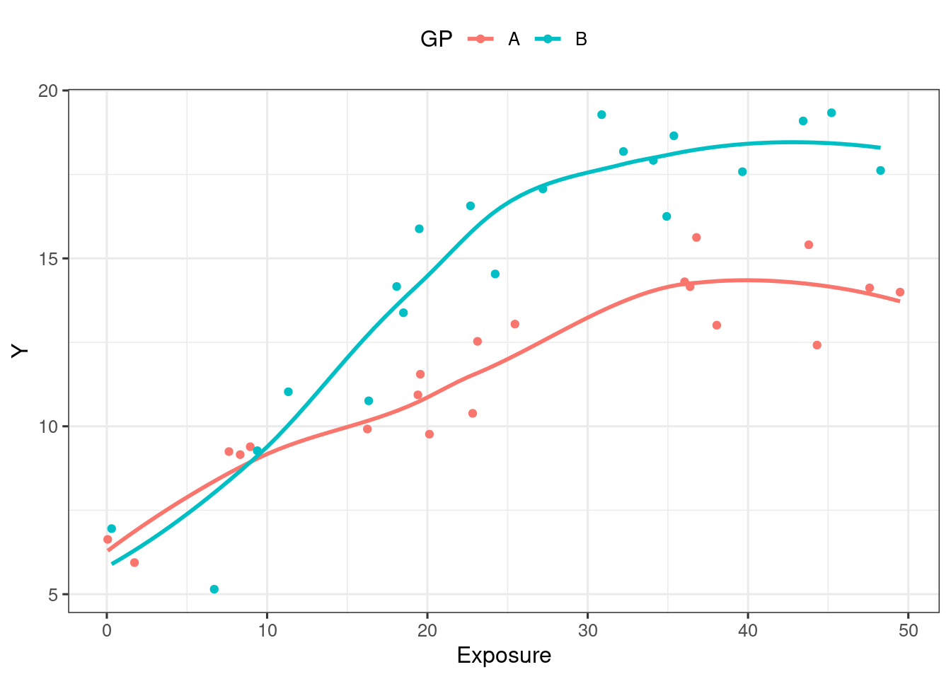
Convenience functions used to generate the data sets. For the purposes of this data set exposures are assumed to be log-normally distributed (with slight truncation) and scale linearly with exposure. Continuous covariates are all bounded between 0 and 10.
emax_fn <- function(exposure, emax, ec50, e0, gamma = 1) {
  e0 + emax * (exposure ^ gamma) / (ec50 ^ gamma + exposure ^ gamma)
}

generate_exposure <- function(dose, n, meanlog = 4, sdlog = 0.5) {
  dose * qlnorm(
    p = runif(n, min = .01, max = .99),
    meanlog = meanlog,
    sdlog = sdlog
  )
}

generate_covariate <- function(n) {
  rbeta(n, 2, 2) * 10
}Define a function make_continuous_data() that simulates exposure-response data for a study with three dosing groups, continuous Emax response, and three continuous covariates:
make_continuous_data <- function(seed = 123) {

  set.seed(seed)

  par <- list(
    emax   = 10,
    ec50   = 4000,
    e0     = 5,
    gamma  = 1,
    sigma  = .6,
    coef_a = .3,
    coef_b = .2,
    coef_c = 0
  )

  make_data <- function(dose, n, par) {
    tibble(
      dose = dose,
      exposure = generate_exposure(max(dose, .01), n = n),
      cov_a = generate_covariate(n = n),
      cov_b = generate_covariate(n = n),
      cov_c = generate_covariate(n = n),
      response = emax_fn(
        exposure,
        emax = par$emax,
        ec50 = par$ec50,
        e0 = par$e0,
        gamma = par$gamma
      ) +
        par$coef_a * cov_a +
        par$coef_b * cov_b +
        par$coef_c * cov_c +
        rnorm(n, 0, par$sigma)
    )
  }

  dat <- bind_rows(
    make_data(dose = 100, n = 100, par = par),
    make_data(dose = 200, n = 100, par = par),
    make_data(dose = 300, n = 100, par = par)
  )

  return(dat)
}
Call the function to generate the data set:
d_example_emax_3cov <- make_continuous_data()
d_example_emax_3cov
# A tibble: 300 × 6
dose exposure cov_a cov_b cov_c response
<dbl> <dbl> <dbl> <dbl> <dbl> <dbl>
1 100 4151. 5.71 2.33 7.83 13.8
2 100 8067. 4.92 4.66 6.74 14.0
3 100 4878. 4.88 4.21 4.68 13.2
4 100 9713. 8.42 6.56 1.29 16.1
5 100 11491. 4.37 3.96 3.55 15.1
6 100 2452. 8.69 7.60 3.64 13.4
7 100 5652. 6.61 3.95 5.13 13.5
8 100 9939. 5.35 7.77 8.29 15.5
9 100 5817. 5.61 2.24 9.60 12.5
10 100 5176. 6.06 1.79 8.74 13.3
# ℹ 290 more rowsScatter plots and loess regressions of response against the four relevant predictors: exposure, cov_a, cov_b, and cov_c:
d_example_emax_3cov |>
  pivot_longer(
    cols = c(exposure, cov_a, cov_b, cov_c),
    names_to = "variable",
    values_to = "value"
  ) |>
  ggplot(aes(value, response)) +
  geom_point() +
  geom_smooth(formula = y ~ x, method = "loess") +
  facet_wrap(~ variable, scales = "free_x") +
  theme_bw()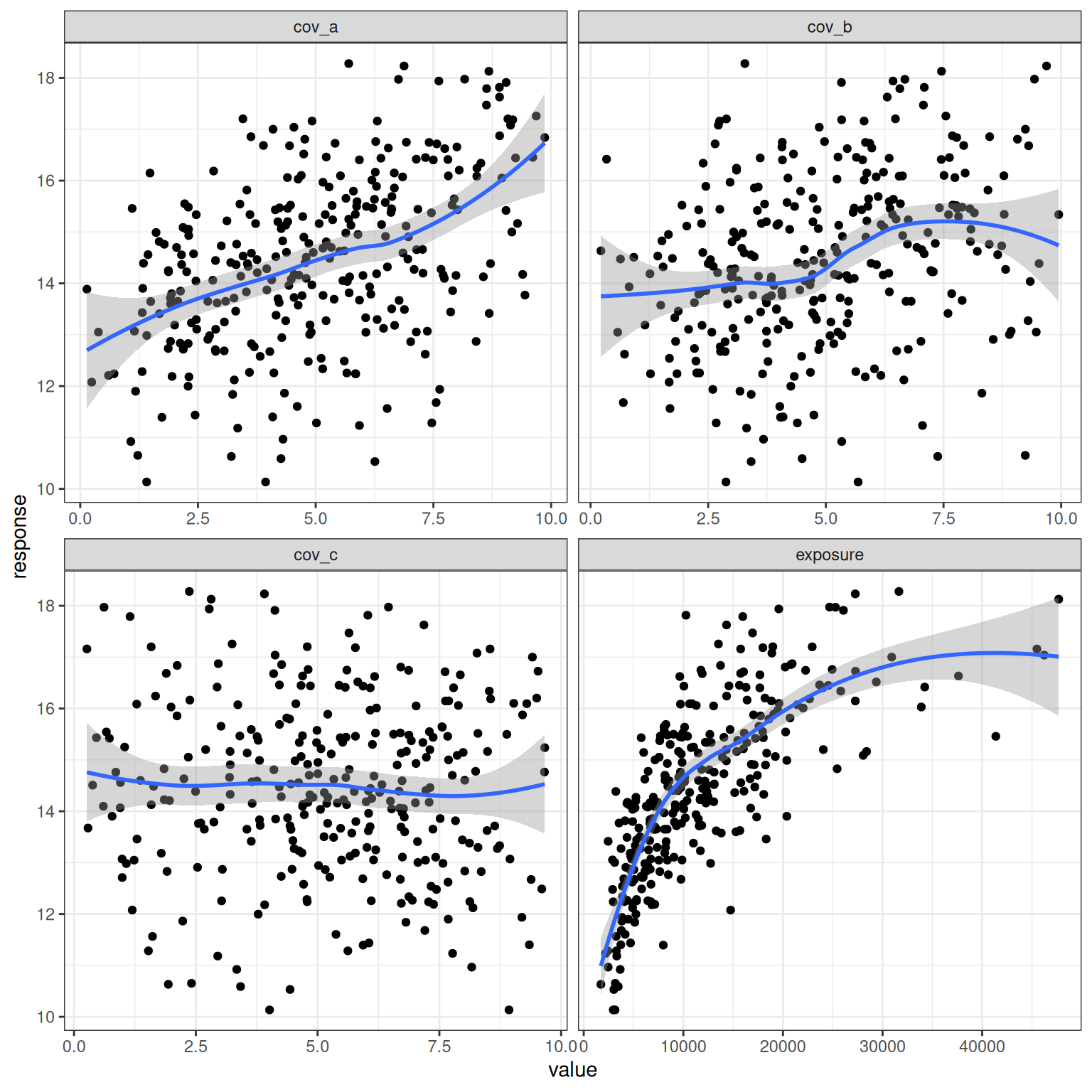
Define a function make_binary_data() that simulates exposure-response data for a study with three dosing groups, binary Emax response, and three continuous covariates:
make_binary_data <- function(seed = 123) {

  set.seed(seed)

  par <- list(
    emax   = 5,
    ec50   = 8000,
    e0     = -3,
    gamma  = 1,
    coef_a = .2,
    coef_b = 0,
    coef_c = 0
  )

  make_data <- function(dose, n, par) {
    tibble(
      dose = dose,
      exposure = generate_exposure(max(dose, .01), n = n),
      cov_a = generate_covariate(n = n),
      cov_b = generate_covariate(n = n),
      cov_c = generate_covariate(n = n),
      pred = emax_fn( # non-linear predictor
        exposure,
        emax = par$emax,
        ec50 = par$ec50,
        e0 = par$e0,
        gamma = par$gamma
      ) +
        par$coef_a * cov_a +
        par$coef_b * cov_b +
        par$coef_c * cov_c,
      prob = 1 / (1 + exp(-pred)), # response probability
      response = as.numeric(runif(n) < prob) # binary response
    ) |>
      select(-pred, -prob)
  }

  dat <- bind_rows(
    make_data(dose = 100, n = 100, par = par),
    make_data(dose = 200, n = 100, par = par),
    make_data(dose = 300, n = 100, par = par)
  )

  return(dat)
}d_example_emax_bin_3cov <- make_binary_data()
d_example_emax_bin_3cov# A tibble: 300 × 6
dose exposure cov_a cov_b cov_c response
<dbl> <dbl> <dbl> <dbl> <dbl> <dbl>
1 100 4151. 5.71 2.33 7.83 0
2 100 8067. 4.92 4.66 6.74 1
3 100 4878. 4.88 4.21 4.68 1
4 100 9713. 8.42 6.56 1.29 1
5 100 11491. 4.37 3.96 3.55 0
6 100 2452. 8.69 7.60 3.64 0
7 100 5652. 6.61 3.95 5.13 0
8 100 9939. 5.35 7.77 8.29 0
9 100 5817. 5.61 2.24 9.60 0
10 100 5176. 6.06 1.79 8.74 0
# ℹ 290 more rowsViolin plots showing the distribution of the four relevant predictors exposure, cov_a, cov_b, and cov_c stratified by whether the response is 0 or 1:
d_example_emax_bin_3cov |>
  pivot_longer(
    cols = c(exposure, cov_a, cov_b, cov_c),
    names_to = "variable",
    values_to = "value"
  ) |>
  mutate(response = factor(response)) |>
  ggplot(aes(response, value)) +
  geom_violin(draw_quantiles = .5) +
  facet_wrap(~ variable, scales = "free_y") +
  theme_bw()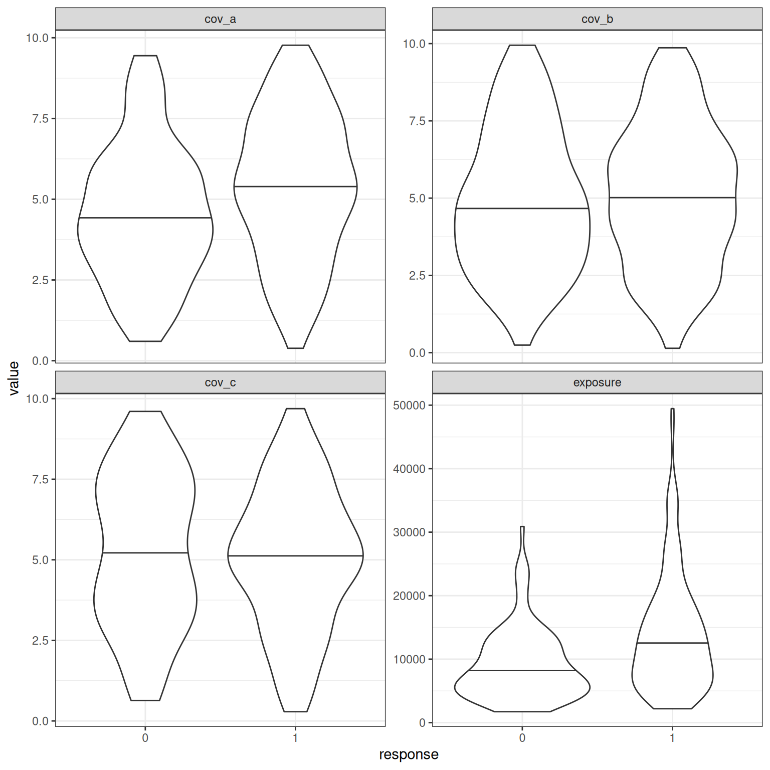
Only run in an interactive session so that the data is not saved every time the document is rendered (by setting eval: FALSE).
write_csv(d_example_emax_nocov, here("data", "d_example_emax_nocov.csv"))
write_csv(d_example_emax_cov, here("data", "d_example_emax_cov.csv"))